Nudging Life Insurance Holdings in the Workplace — Journal article

Authors: Timothy F. Harris and Aaron Yelowitz
Citation: Timothy F. Harris and Aaron Yelowitz (2017). Nudging Life Insurance Holdings in the Workplace. Economic Inquiry 55(2): 951–981. DOI: 10.1111/ecin.12390.

This supplied published online-first article uses pages 1–31.

Abstract

Using data from a university, we analyze a policy designed to increase employer-sponsored life insurance. The university increased basic life insurance holdings, which nudged employees with supplemental coverage to have more life insurance. In large part due to inertia, the nudge increased life insurance holdings one-for-one for those who could have undone it. Additionally, we find that expanding coverage options significantly increased total life insurance holdings for new hires who were not subject to inertia. These policy changes reduced uninsured vulnerabilities for two-thirds of employees. Our findings have important policy implications for addressing widespread disparities in life insurance coverage.

JEL classification: D31; G22; D03; J32; J33; J38; H20
Affiliations: Timothy F. Harris — Ph.D. Candidate, Department of Economics, University of Kentucky, Lexington, KY 40506 (tim.harris@uky.edu); Aaron Yelowitz — Associate Professor, Department of Economics, University of Kentucky, Lexington, KY 40506 (aaron@uky.edu).
Acknowledgments: We thank Frank Scott, Glenn Blomquist, John Garen, William Hoyt, Chris Bollinger, Anthony Creane, Tom Ahn, Kitt Carpenter, Adib Bagh, Jim Marton, Jose Fernandez, Jeremiah Harris, David Agrawal, Alyssa Harris, participants at University of Kentucky and Vanderbilt VEAM conferences, and anonymous referees for comments and Matthijs Schendstok for research assistance.

I. INTRODUCTION

Life insurance ownership is at a 50-year low and sales have declined 45% since the mid-1980s (Prudential 2013; Scism 2014). Large disparities exist between life insurance holdings and underlying vulnerabilities with some estimates exceeding $15 trillion (Bernheim et al. 2003; Conning, Inc. 2014; LIMRA 2015b). These disparities are partially explained by many individuals’ inability to correctly answer rudimentary financial questions and difficulties associated with thinking about death and gauging mortality risk (Kopczuk and Slemrod 2005; Lusardi and Mitchell 2006, 2007).

Notwithstanding these disparities, 70% of households have some form of life insurance coverage, which is split between individual and group markets. The two markets differ in that individual market premiums are experience rated with extensive underwriting, while group markets typically have some form of community rating and guaranteed issue. Previous work has focused almost exclusively on the individual market (Cawley and Philipson 1999; Harris and Yelowitz 2014, 2015; He 2009, 2011; Hedengren and Stratmann 2016). Little attention, however, has been given to the group or employer-sponsored life insurance (ESLI) market where 39% of households have coverage.

In a recent paper on behavioral economic interventions, Madrian (2014) proposed prompting individuals to make a concrete plan to elect life insurance in order to increase coverage. A different approach to address uninsured vulnerabilities is through an increase in employer provision. As with any type of employer or government provision, there is the principal concern of crowd-out. A growing literature, however, documents considerable levels of inertia that lessens the crowd-out effect (Chetty et al. 2014; Handel 2013; Thaler and Sunstein 2008).

We use administrative data from a large public university (“the University” henceforth) with approximately 16,000 employees to analyze the impact of increased employer provision of life insurance on total life insurance coverage. There are two types of ESLI available for employees at the University: basic, which is automatically provided by the employer, and supplemental which is available in multiples of salary.

Abbreviations

ACS: American Community Survey
ESLI: Employer-Sponsored Life Insurance
FSA: Flexible Spending Account
LTD: Long-Term Disability
NCS: National Compensation Survey
SIPP: Survey of Income and Program Participation

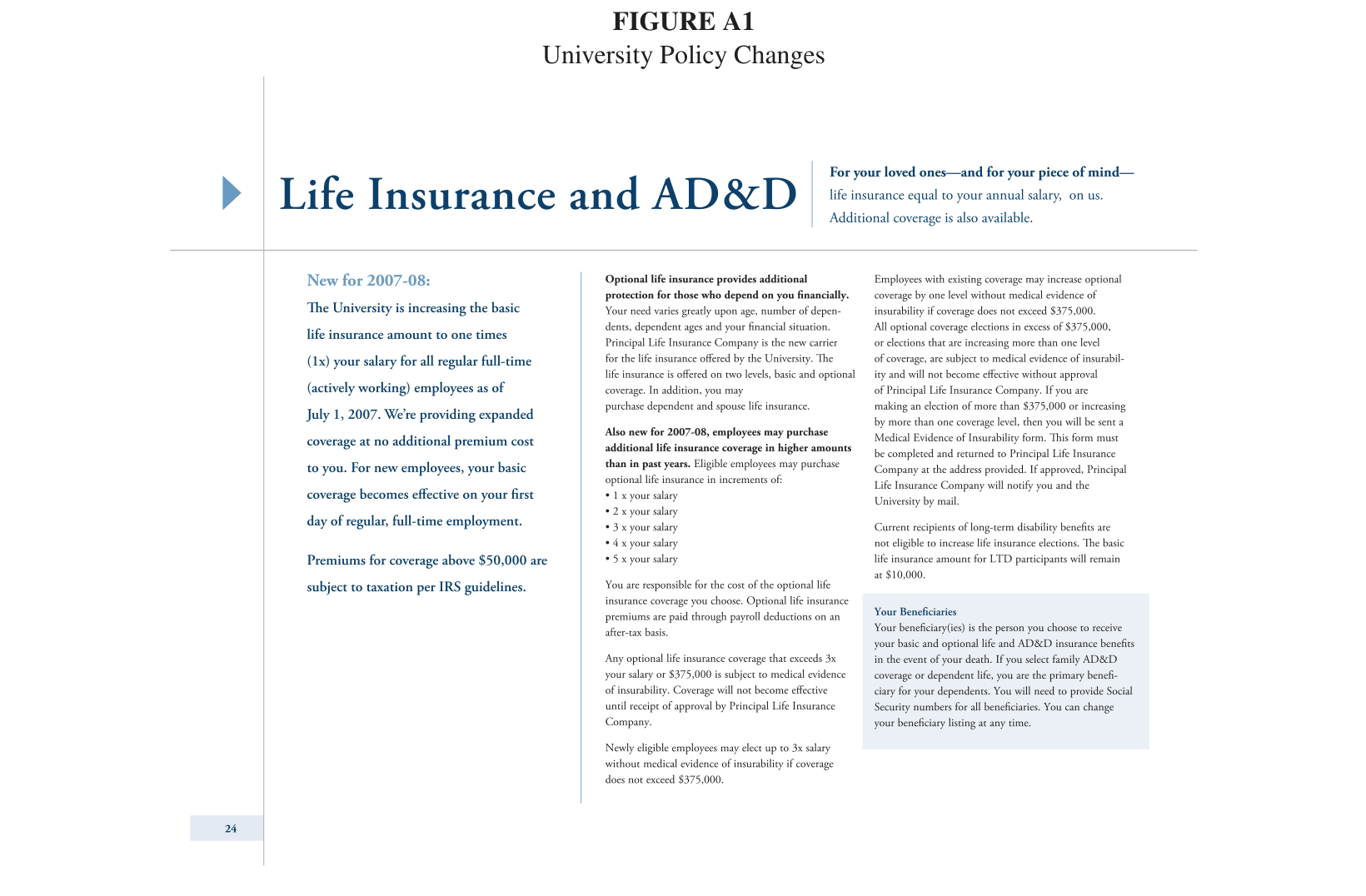
In 2008, the University increased provision of basic life insurance coverage from $10,000 to 1× the worker’s annual salary and increased the maximum coverage from $375,000 to $1 million. For existing employees, the choice of supplemental coverage remained at the default level chosen in 2007; to undo the nudge to increase total coverage, an employee would actively have to scale back supplemental coverage. The neoclassical model predicts one-for-one crowd-out for those electing supplemental coverage in 2007.

Using two distinct samples, we observe considerable levels of inertia. The first group we analyze consists of existing employees who elected a multiple of 1× or 2× salary (interior) in 2007 (1,867 employees). These individuals were in a position to completely undo the increase in basic coverage and were not constrained by a maximum contribution limit. For example, an employee with 1× salary in supplemental coverage making $60,000 would experience an increase in total coverage from $70,000 to $120,000 (1.17–2× salary) if they did not reduce supplemental coverage. For this sample, we find full pass-through of the increase in basic coverage with a precisely estimated 97% pass-through as a lower bound.¹ Full pass-through is found in both the short and long run and for every demographic group. The second group contains highly compensated employees (making $125,000 to $187,500) who were constrained by the maximum contribution limit in 2007 and who chose supplemental coverage worth 3× salary (86 employees). Owing to the $375,000 maximum, they were effectively assigned a multiple less than 3× salary. For example, an employee making $160,000 (who elected 3× salary) was constrained to have only 2.34× salary ($375,000) in supplemental coverage. The policy change automatically increased both basic coverage as well as supplemental coverage from 2.34× to 3× salary. In the case of full inertia, this policy change increased total coverage from 2.4× to 4× salary ($385,000 to $640,000). Over 75% of this group did nothing in response to this change consistent with inertia.

New employees, however, are not influenced by inertia because they are required to complete a form where they name a beneficiary and make an active decision regarding the multiple of salary for supplemental ESLI. For new hires, we find that a $100 increase in basic life insurance coverage decreases supplemental coverage by $23. The reduction in supplemental coverage for those without the influence of inertia is consistent with partial crowd-out. Therefore, we conclude that inertia in part drives the full pass-through of the increase in basic coverage for existing employees.

Potential reasons why we do not find full crowd-out of the increase in basic coverage for new hires include context effects, implicit advice, and flypaper effects. Individuals tend to elect the middle option due to compromise effects and avoidance of extremes (Kamenica 2008; Simonson 1989; Simonson and Tversky 1992). Consequently, the expansions of the maximum face value (from $375,000 to $1,000,000) and the available multiples of coverage (from 0–3× to 0–5× salary) could have increased new hire supplemental elections. Employees could have also interpreted the expanded options as implicit advice to increase supplemental ESLI coverage. Additionally, Choi, Laibson, and Madrian (2009) find that employees fail to take into account the allocation of employer contributions when choosing their own allocations for 401(k) accounts. It could be the case that employees partially fail to take into account employer contribution when determining their level of supplemental ESLI coverage thus leading to less than full crowd-out for new hires.

Even though we do not find crowd-out of the perfect substitute, supplemental ESLI, for existing employees, it is possible that employees reacted to the increased provision of basic coverage by decreasing an imperfect substitute, individual life insurance (term or whole life policies). We cannot directly observe this response for the University’s employees, so we use the Survey of Income and Program Participation (SIPP) and a quasi -experimental approach that examines job switchers to identify the effect. Even among job switchers, who should be the most responsive, we find little substitution between employer-sponsored and individual markets with less than 1 in 10 workers changing individual coverage in reaction to changes in ESLI. If University employees react in a similar fashion, then increases in ESLI coverage, by and large, represent increases in total life insurance holdings.

Overall, the nudge was effective in the sense that it increased life insurance coverage, but was it a sensible nudge? We analyze how employees’ holdings relate to the recommended levels of life insurance coverage. In 2007, approximately two-thirds of employees were below recommended levels and the remainder were above.

The increased provision of basic coverage reduced the average disparity between actual and recommended coverage. Of those with adequate coverage prior to the increase, over 90% had no dependents and consequently had little need for coverage. In addition to analyzing the effectiveness of the increase in basic coverage to 1 × salary, we explore alternative expenditure neutral policies. We find that equal contributions to premiums mitigate disparities better than multiples of salary or fixed coverage amounts.

This article contributes to the body of literature on inertia. Researchers have analyzed inertia on the extensive margin related to default participation in 401(k) plans (Choi et al. 2002, 2004; Madrian and Shea 2001) and organ donation (Abadie and Gay 2006; Johnson and Goldstein 2003). Additional research has explored inertia on the intensive margin in the context of Medicare Part D choice (Ericson 2014), retirement contribution (Chetty et al. 2014; Messacar 2014), private health insurance choice (Handel 2013), income tax refunds (Jones 2012), and Medicaid plan choice (Marton and Yelowitz 2016). This study primarily examines the intensive margin where employees first choose coverage and then encounter frictions that lead to inertia despite a changing default.

Although inertia and pass-through have been found in previous studies as outlined above, the degree of inertia varies significantly depending on the context. For example, Chetty et al. (2014) find that 85% of employees are passive (inert) and save more due to increased automatic retirement contributions, whereas Dahl and Forbes (2016) find in the context of health insurance that only 16% of employees are inert 1 year after the policy change. Benefits that are used more frequently or are more salient (i.e., carry a greater financial cost) are harder to nudge. Life insurance represents a small budget share and payouts are received only in the case of a low probability event. Therefore, it is unlikely that the degree of inertia for ESLI would be equivalent to findings in other markets. The sheer magnitude of inertia and not merely its existence is important for policy makers seeking to address widespread uninsured vulnerabilities in life insurance coverage.

The remainder of the article is organized as follows. Section II describes the policy change and theoretical predictions. Section III describes the data and representativeness of the University sample. Section IV provides the empirical specification. Section V presents our results. Section VI analyzes the relationship between the individual and non-group markets.

Section VII explores the desirability of the nudge and alternative policies. Section VIII concludes.

II. POLICY CHANGES AND THEORETICAL PREDICTIONS

Prior to detailing the policy change at the University, we present a simplified model to describe a representative agent’s choice of supplemental life insurance coverage given basic coverage provided by an employer. In the model, the individual chooses supplemental ESLI coverage, $d_{S}$ , and pays an actuarially fair premium.² After choosing coverage and paying the corresponding premium, the employee either dies and her family receives a payout or she lives and receives an income stream, y. The utility maximization problem is given by the following objective function:

Equation 1. Maximize V over supplemental coverage dS: (1−rho) U(y+w−rho dS−rho dB) + rho U(w−rho dS−rho dB+dS+dB). The two terms weight utility in survival and death states. — Equation 1. Open full-resolution image.

where $U (\cdot)$ represents a concave utility function, $ρ$ is the probability of death, and w is wealth (transferable). Payouts are given by $d_{S}$ and $d_{B}$ , respectively, for supplemental and basic coverage. In this model, we assume that employees bear the cost of basic ESLI. Nonetheless, the results do not change if the employer merely gives the employee’s dependents $d_{B}$ in the case of the employee’s death.³

The basic optimization problem leads to the familiar result of full insurance with $d_{S}^{*} = y - d_{B}$ . As is apparent from the solution, supplemental coverage should decrease one-for-one as basic coverage increases for those at an interior solution. If $d_{S}^{*}$ is zero, then employees cannot reduce coverage in response to increases in basic coverage. Additionally, if $d_{S}$ is constrained to be below $d_{S}^{*}$ , then employees should not decrease coverage with an increase in basic ESLI inasmuch as the increase does not exceed the optimal level of total insurance. The main result, for those at an interior solution, is one-for-one crowd-out of supplemental coverage with an increase in basic coverage.

In 2008, the University increased basic coverage from $10,000 (0.18× salary on average) to 1× annual base salary for all qualified employees.⁴⁵ This increase in basic coverage, given no employee response, results in an increase of life insurance of approximately 1× the employees’ annual salary. The increase in basic coverage is crucial for understanding the responsiveness of employees to changes in life insurance coverage. In the absence of the increase in basic coverage, preferences and needs for life insurance evolve slowly over time and lead to relatively few changes in supplemental coverage. Additionally, ESLI automatically adjusts for changes in income because coverage is elected in multiples of salary. In the year preceding the increase in basic coverage, 90% of employees with supplemental ESLI kept the same level of coverage. The lack of change in the year before cannot be deemed inertia because preferences and needs for coverage likely did not sufficiently change in a single year to merit adjustments to supplemental coverage. On the other hand, increased provision of life insurance should elicit a response.

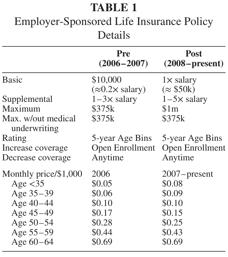
Table 1 outlines the life insurance parameters both before and after the increase in basic coverage.⁶ Qualified employees could always elect supplemental life insurance in multiples of annual salary. Although near ubiquitous in the individual life insurance market, health screening has a minimal role in ESLI. At the University, health screening is only required for supplemental coverage over $375,000 or for large jumps in coverage.⁷ Premiums on supplemental life insurance are community rated and assigned based on 5-year age bins, which workers pay on an after-tax basis through payroll deductions. Premiums changed between 2006 and 2007 and then remain unchanged for the duration of the sample. Premiums increased by 60% and 50% for those aged 18–34 and 35–39 years, respectively. The increased premiums could have caused employees to reduce coverage.⁸ If there were a lagged effect—employees react the following year—then this would indicate crowd-out of the increase in basic coverage when it was the result of changing premiums. Therefore, for those under age 40, our analysis will overstate crowd-out. In 2007, employees were required to resubmit a life insurance elections form to update beneficiaries. The forced recalibration of ELSI made the price change more salient and if employees wanted to alter supplemental coverage, they likely would have done it in 2007. Regardless, we use older employees who did not experience a premium change to verify the robustness of our findings.

As illustrated in Table 1, prior to 2008, qualified employees could elect supplemental life insurance at multiples of 1–3× base salary up to a maximum of $375,000.⁹ Beginning in 2008, the multiple limits were expanded to include 4× and 5× annual salary with a $1 million maximum contribution limit. The increased maximum election should only affect those individuals who elected 3× annual salary prior to 2008 or those constrained by the $375,000 maximum.

Table 1. Employer-Sponsored Life Insurance Policy Details

Table 1. Employer-sponsored life insurance before and after the 2008 policy change: basic coverage rises from $10,000 to one times salary and supplemental options from one–three to one–five times salary. Rows also report maximum coverage, underwriting, enrollment rules, and monthly prices per $1,000 by age. — Table 1. Open full-resolution image.

Although the simplified representative agent model predicts full crowd-out of increased basic ESLI, it does not perfectly describe the situation at the University. Owing to the restriction of selecting whole multiples of supplemental coverage and given that the increase is not exactly the same as a multiple of supplemental coverage, it is possible that nonresponse is optimal for some individuals. For example, suppose the optimum for an individual is total ESLI of 2× salary. Prior to 2008, the individual selects 1× salary in supplemental coverage if $V (1 x + $ 10 k) > V (2 x + $ 10 k)$ . After 2008 the individual has 2× salary in total coverage due to the increase in basic coverage and optimally does not reduce supplemental coverage because $V (2 x) > V (1 x)$ . Although possible, this scenario likely only applies to a small minority of employees.¹⁰ Additionally, the likelihood of this scenario should decrease for higher earners where $10,000 in coverage represents a smaller proportion of total coverage.

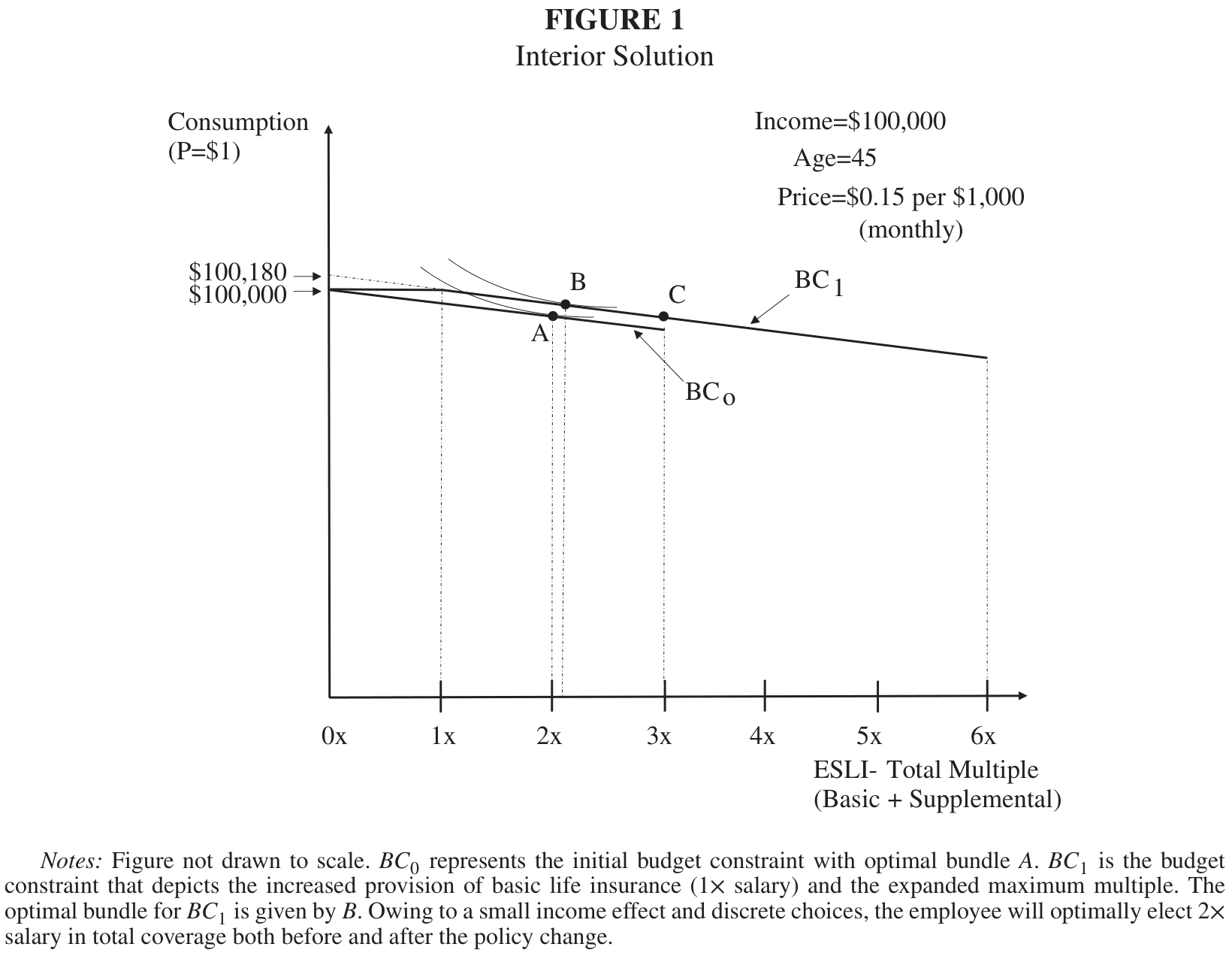
We illustrate the increase in basic coverage and the expanded maximum in Figure 1 assuming that employees are utility maximizers and that life insurance is a normal good. This figure depicts the life insurance decision for a 45-year-old employee with an annual income of $100,000. Prior to the policy change, individuals faced budget constraint $B C_{0}$ and optimally choose bundle $A$ , which consists of total life insurance coverage worth 2× annual salary. After the policy change, employees were subject to $B C_{1}$ , which incorporates the provision of 1× salary in basic coverage and the increase in available multiples. If an employee does not react to the changing budget constraint, she ends up at point $C$ with increased life insurance coverage. Optimally, the employee selects bundle $B$ but due to the restriction of purchasing whole multiples of coverage the individual continues with 2× salary in total ESLI coverage. Therefore, for this interior solution, the increase in basic life insurance from essentially 0× to 1× salary is completely offset due to one-for-one crowd-out such that the individual optimally demands the same level of total coverage.

There is a minimal increase in total compensation—on the order of 0.2%—from this increase in basic coverage, which leads to a tiny income effect.¹¹ The average worker receives a $121 annual increase in total compensation because of the increase in basic coverage (based on supplemental premiums). Employees likely pay for the increase in coverage in the form of smaller raises or bonuses. Inasmuch as employees recognize this implication, the tiny income effect only decreases. Therefore, the likely prediction is one-for-one crowd-out and no increase in total life insurance holdings for those with 1–2× salary in 2007.

A possible explanation for any lack of response is that the initial supplemental ESLI election became suboptimal over time due to changing needs or acquired information indicating a need for more coverage. If this were the case, the increase in basic coverage reflected a costless adjustment to an optimum that individuals did not undertake themselves due to time costs of updating supplemental coverage. However, as previously mentioned, all employees in 2007 were required to fill out a life insurance form to update beneficiaries. Included on the same one-page form was the option to change supplemental coverage by merely checking a box. Therefore, if employees had latent demand for more coverage, there was a virtually costless opportunity to increase coverage the year before the increase in basic coverage making the scenario less likely.

Figure 1. Interior Solution

Notes: Figure not drawn to scale. $B C_{0}$ represents the initial budget constraint with optimal bundle $A$ . $B C_{1}$ is the budget constraint that depicts the increased provision of basic life insurance (1× salary) and the expanded maximum multiple. The optimal bundle for $B C_{1}$ is given by $B$ . Owing to a small income effect and discrete choices, the employee will optimally elect 2× salary in total coverage both before and after the policy change.

Failure to observe crowd-out for employees at the interior solution (i.e., 1× or 2×) could be a result of employee inattention or lack of understanding. The University mails benefit booklets to employees, which inform them of changes and benefit availability (see Appendix A). This information is also available through the Human Resource website. Nonetheless, it is possible that employees were unaware of the increase in basic coverage or did not understand that supplemental elections would remain the same. Later, we use overall activity and changes in other benefits to infer awareness.

An alternative explanation for not finding crowd-out could be prohibitively expensive costs of changing coverage. Various psychological frictions or costs exist that could cause deviations from the rational frictionless model. Implicit costs due to the difficulty of evaluating the relative advantages for the various types of life insurance can decrease coverage (Handel 2013; Iyengar, Huberman, and Jiang 2004). Furthermore, the psychological cost of thinking about death decreases the likelihood of changing life insurance elections (Kopczuk and Slemrod 2005). In addition, employees needed to submit a paper form to the benefits office to decrease supplemental coverage, which represents a time cost for changing the policy. We account for this time cost by analyzing employees that made simultaneous changes to other benefits and consequently have reduced costs for making an additional change to supplemental life insurance.

Even though our analysis primarily focuses on those at the interior, it is important to understand the response of employees at the corners when considering the overall impact of the increase in basic coverage. For individuals who did not elect supplemental coverage, the increase in basic coverage mechanically increases (“shoves”) total coverage from $10,000 to 1× annual salary. Any change in total coverage above 1× salary could be due to perceived implicit advice from the employer or referencing coverage based on the available maximum. For those at 3× salary in 2007, it is likely that they were constrained by the maximum and have latent demand for more coverage. As the available multiple increases from 3× to 5× in 2008, they likely elect more coverage. However, if 3× salary was the desired level of coverage then they should experience complete crowd-out of the increase in basic coverage.¹²

III. DATA

A. Description

We use administrative (payroll) panel data from the University from 2006 to 2014.¹³ The data document complete benefit and retirement elections. Employees make benefit elections during the open enrollment period for the University or after a qualifying event, which include birth, adoption, marriage, divorce, or employment status change.¹⁴ All elections made during the open enrollment period take effect July 1 and continue until a new election in made. In general, employees cannot add or drop coverage during the year except in the case of a qualifying event. Supplemental life insurance is distinct from other benefits in that an employee may reduce insurance coverage at any time.

If an employee leaves the University for any reason, his or her coverage for either basic or supplemental life insurance lapses unless the individual qualifies for long-term disability (LTD) or the employee dies within 3 months.¹⁵ This lock-in aspect of ESLI is contrasted with individual market coverage, which is contingent on premium payments alone and not employment. Evidence of lock-in has been shown in employer-sponsored health insurance and cliff vesting for defined benefit pensions (Kotlikoff and Wise 1987; Madrian 1994).

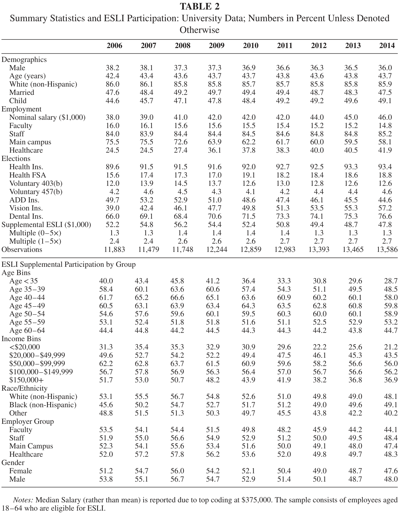
Table 2 shows the summary statistics for 23,132 unique workers from 2006 to 2014 who are eligible for supplemental life insurance coverage. The sample is predominantly female (63%) and white (86%). Roughly half of the sample is married and over 40% of the sample has a child.¹⁶ Faculty make up less than 20% of the sample. In addition to the main campus, the University operates a hospital. The relative employment share for healthcare increased 17 percentage points over the period; all healthcare workers are classified as staff.¹⁷ The data report annual base salary in thousand dollar increments top coded at $375,000. Median salary increased in nominal terms from $38,000 to $46,000 over the 9 years of the sample. This value does not take into account bonuses, raises that occur during the year, or summer ninths.

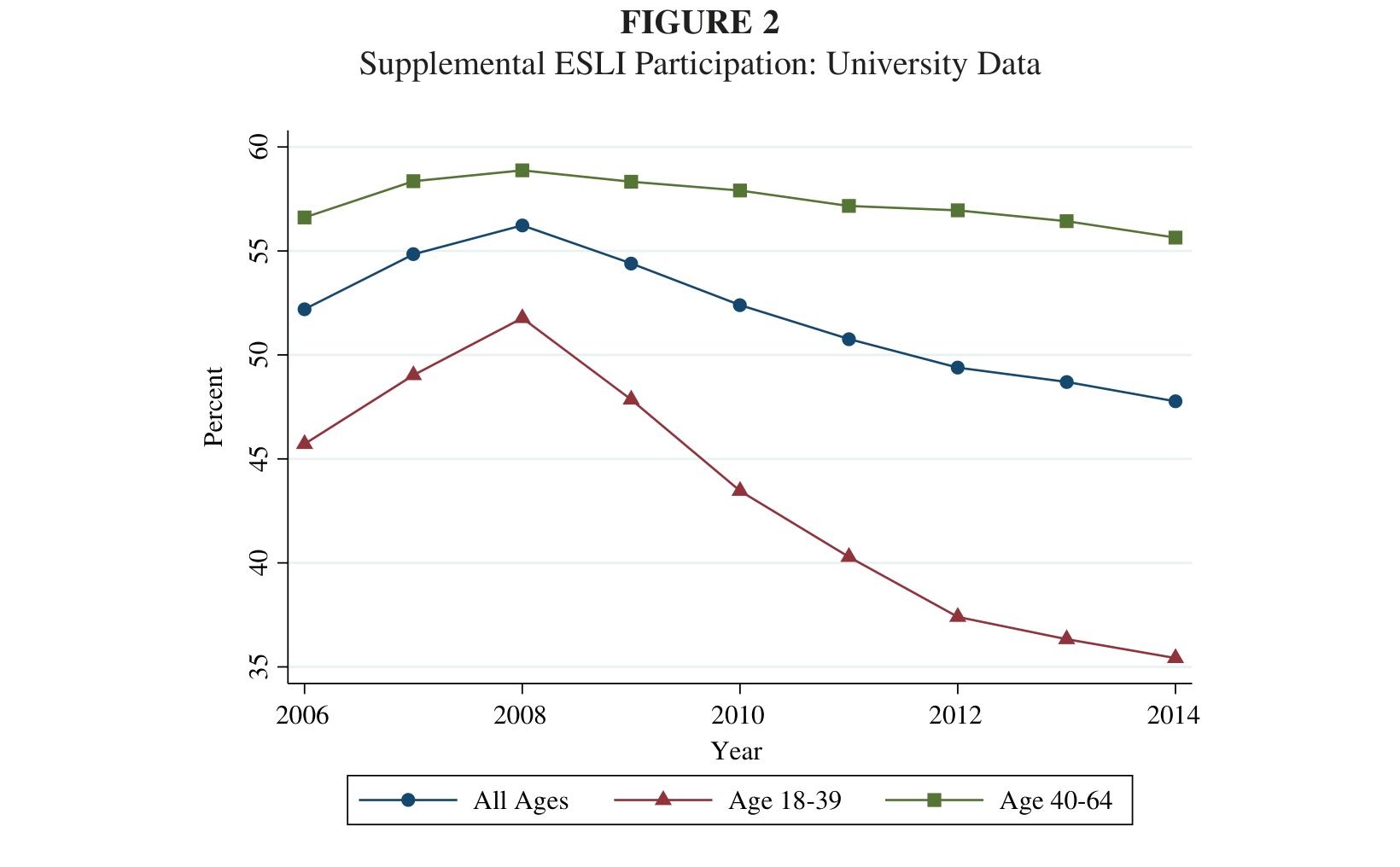
Figure 2 shows that supplemental participation increased until 2008 and then decreased from 56% to 48% in the course of 6 years for all employees. However, this decline is not present for continuously employed workers. This indicates that the decrease in supplemental participation is driven by new hires. Generally, we do not observe new hires in the data until the year following their hire date as many were hired during the fiscal year.¹⁸ Therefore, as shown in the figure, the decline in participation begins a year later than would be expected from crowd-out due to the lagged observation of new hires.

Table 2. Summary Statistics and ESLI Participation: University Data; Numbers in Percent Unless Denoted

Table 2. University data for 2006–2014: demographic and employment characteristics, benefit elections, supplemental insurance amounts and participation by age, income, race, employment group and gender. Columns are years; sample sizes and the median-salary/sample note are included. — Table 2. Open full-resolution image.

The second panel of Table 2 breaks out supplemental life insurance participation by different demographic groups. The participation profile is hump shaped with respect to age and peaks between ages 40 and 45. Life insurance’s primary purpose is to replace the lost earnings of a breadwinner, which means as the individual approaches retirement demand might decrease as potential lost earnings decrease. For employees under age 55, participation rates increased from 2006 to 2008 and then consistently fell for the remainder of the sample. For those under age 35, participation dropped from 46% in 2008 to 29% in 2014. No decline exists for employees older than 50.

Table 2 further shows how income levels influence participation. For employees that make less than $100,000, there is the same trend of increasing participation up to 2008 followed by steady significant decline. This trend exists for faculty, staff, main campus, and healthcare employees. Faculty are less likely to hold supplemental ESLI in comparison to staff for every year except 2006. This perhaps could be the result of differential participation in the individual term life insurance market. There are no significant gender differences.

Figure 2. Supplemental ESLI Participation: University Data

Figure 2. Supplemental employer-sponsored life insurance participation, 2006–2014. All-age participation peaks near 56 percent in 2008 and falls to about 48 percent in 2014. The decline is larger for ages 18–39 than for ages 40–64; all three series and their legend are shown. — Figure 2. Open full-resolution image.

B. Representativeness

Many universities publish online benefits booklets through their human resource offices with varying degrees of detail on fringe benefits, including ESLI. We collected benefits booklets in 2014 from more than 400 institutions. Of these, we select 70 institutions that have well-documented information on both basic and supplemental life insurance coverage. The benefit booklets for many institutions were missing details on life insurance and we are hesitant to conclude that such institutions do not offer coverage. Nearly 70% of employees across all occupations are offered life insurance coverage, and the take-up rate is 80%. Additionally, half of all employees are offered supplemental coverage (LIMRA 2015a).

Although many differences exist across universities with respect to their provision of life insurance, several common features emerge for the 70 institutions examined. First, premiums are community rated, often with 5-year age bins, similar to the University in this study. Virtually all institutions have an open enrollment period where new employees can purchase coverage without underwriting and where the issuance of policy is guaranteed.

Second, a large majority of basic plans are provided as a multiple of salary. Of the 70 plans, 30% had basic coverage at 1× salary, 17% at 1.5× salary, and 24% at 2× salary. Thus, the University’s design of its basic plan from 2008 onward is representative of a much larger set of institutions, both in terms of structure and generosity. Almost all of the remaining plans (12 of the 20 that were not multiples at 1×, 1.5×, or 2× salary) offered a flat dollar amount of coverage, most often in the range of $20,000 to $50,000. Such flat dollar life insurance plans mimic the basic structure at the University prior to 2008 (where the flat dollar amount of $10,000 was considerably lower than most plans).

Third, almost half of institutions scale back basic life insurance coverage once employees reach a threshold age, often 65 or 70. Relative to younger employees, the payout typically falls by at least 35%. In 2008, the University adjusted the coverage such that payouts fell to a flat amount of $10,000, rather than 1× salary, once an employee reached age 70.

Fourth, three-quarters of supplemental plans also offer coverage in multiples of salary, with maximum payouts that will be binding for higher-paid employees. The most common maximum multiple is 5× salary, with a range from 2× to 10× salary. The University’s change in 2008 brought the supplemental maximum in line with other universities. The remaining one-quarter of supplemental plans offer flat dollar amounts, which allows lower paid employees to purchase far greater multiples of their salary. The most common flat dollar amount is $500,000.

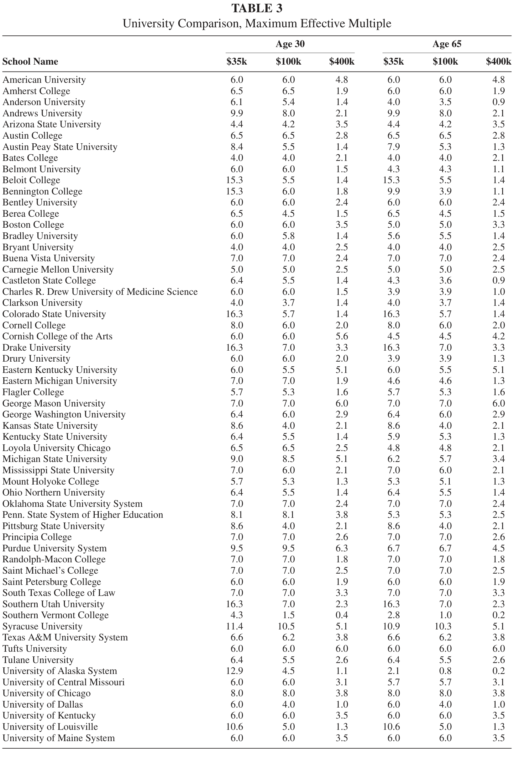
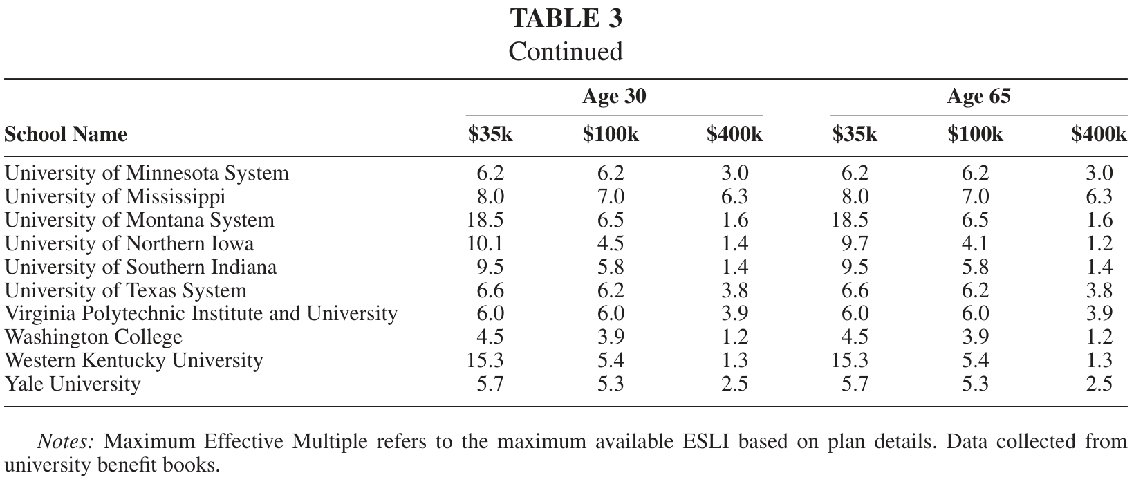
Table 3 combines and summarizes some of the salient features for the 70 universities into a maximum “effective salary multiple” (i.e., total coverage divided by salary). The combination of basic and supplemental plans, multiples of salary and flat dollar amounts, age adjustments, and maximum payouts has implications for the degree of total coverage that an employee can obtain from ESLI. We present the effective salary multiple for three types of earners ($35k, $100k, and $400k) and two ages (age 30 and age 65). Several findings emerge. Lower compensated employees typically have the potential to replace more of their salary through life insurance, both due to plans with flat payout and binding maximums on higher-paid employees. The median effective multiple is 6.5× salary for young employees making $35k, 6.0× salary for those making $100k, and just 2.2× salary for those making $400k. Second, because the majority of plans do not have steep drop-offs based on age, the medians are similar for 65-year-olds, but in some cases, the drop-offs can be quite substantial. For example, a 65-year-old at Michigan State University making $100k can replace just 5.7× her salary, while a 30-year-old can replace 8.5× her salary. The University considered in this study, after the policy change, falls below the median effective salary multiple for most employees.

Table 3. University Comparison, Maximum Effective Multiple

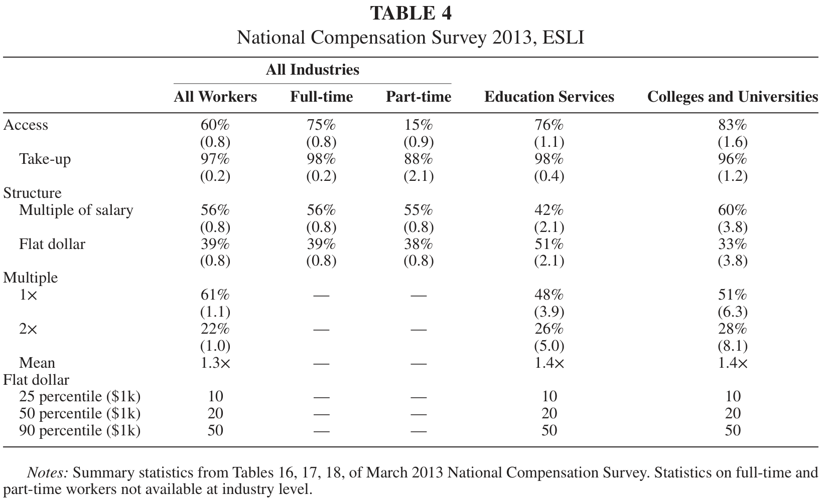
Table 3, first part. Maximum effective life-insurance multiples by university, American University through the University of Maine System. Six columns compare ages 30 and 65 at salaries of $35,000, $100,000 and $400,000; remaining universities follow in the continued panel. — Table 3. Open full-resolution image.

Table 3, continued. Maximum effective life-insurance multiples from the University of Minnesota System through Yale, for ages 30 and 65 and three salary levels. The note defines the maximum multiple and identifies university benefit books as the data source. — Table 3. Open full-resolution image.

The University can also be compared to the more systematic collection of data from the March 2013 National Compensation Survey (NCS) (Bureau of Labor Statistics, U.S. Department of Labor 2013). Evidence is presented in Table 4. Across all industries, 60% of employees have access to ESLI, and take-up of the benefit is virtually complete. Employees in higher education have far greater access to ESLI, and access is higher still at the University. Consistent with the sample of 70 institutions, the most common form of ESLI is as a multiple of earnings, which is approximately twice as prevalent as flat dollar contributions. In addition, for ESLI plans that are designed as a multiple of salary, almost twice as many cover employees at 1× salary as at 2× salary. Among flat dollar plans, the median payment is $20,000, somewhat lower than the sample of 70 institutions.

In summary, data collected from benefits booklets and from the NCS suggest that the University made changes in 2008 that brought its life insurance offering from below average to the norm for colleges and universities. The NCS demonstrates that colleges as a whole tend to be more generous than other industries in the provision of ESLI, but the design of the University’s plan—as a multiple of 1x earnings—is quite common for a broad range of workers. Given these findings, it is likely that the University increased basic ESLI coverage to align itself with industry standards rather than to satiate the changing preferences of existing employees.¹⁹

Table 4. National Compensation Survey 2013, ESLI

Table 4. The 2013 National Compensation Survey: employer-sponsored life-insurance access, take-up, salary-multiple and flat-dollar benefit structures. Columns compare all workers, full-time and part-time workers, education services, and colleges/universities; standard errors and unavailable values are retained. — Table 4. Open full-resolution image.

IV. EMPIRICAL STRATEGY

A. Existing Employees at the Interior

To test the influence of inertia, we restrict the analysis to those employees that elected either 1× or 2× annual salary in 2007 (interior solution) for whom the increase in basic coverage represents a nudge.²⁰ The simultaneous increase in the available multiples from 3× to 5× coverage should not influence this population since by revealed preference they demanded a multiple lower than the maximum. In addition, they have the flexibility to reduce supplemental coverage to offset the increase in basic coverage. This group constitutes 23% of the sample of existing employees. We use the following fixed effects specification to test the effect of the increase in basic coverage.

Equation 2. Total Coverage for individual i at time t equals beta1 times Post at t, plus beta2 times X at i,t, plus individual effect alpha i and error epsilon i,t. — Equation 2. Open full-resolution image.

{T o t a l C o v e r a g e}_{i t}

represents the total coverage (basic + supplemental) in multiples of income for individual $i$

at time $t$

, $X_{i t}$

is a vector of covariates that vary across time (income, age, and main campus vs. healthcare assignment), and ${P o s t}_{t}$

is an indicator variable equal 1 for years following the increase in basic coverage. If $β_{1}$

is zero, then there is no evidence of inertia. The individual fixed effect, $α_{i}$

, controls for unobserved heterogeneity such as risk aversion, latent health, human capital, and underlying needs.²¹

B. New Hires

Next, we analyze the effect of the increase in basic coverage for new hires. Several studies have shown that new hires respond more to changes in benefit pricing and more frequently elect new options relative to existing employees (Handel 2013; Royalty and Solomon 1999; Samuelson and Zeckhauser 1988; Strombom, Buchmueller, and Feldstein 2002). New hires at the University are required to actively choose (no default) if they want supplemental coverage or just basic coverage in addition to listing a beneficiary for basic life insurance.²² Therefore, in the absence of inertia, new hires should have been less likely to opt into, and choose lower levels of, supplemental coverage after the increase in basic coverage.

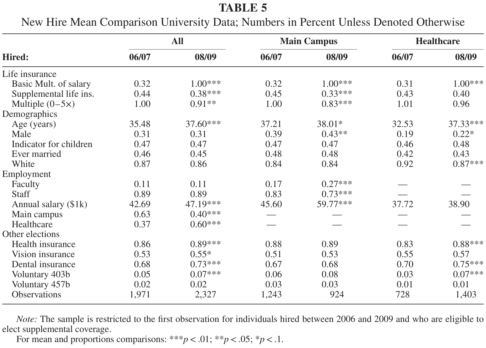
Summary statistics for cohorts of new hires within 2 years of the increase in basic coverage (4,298 employees) are presented in Table 5. The difference in the basic life insurance multiples mechanically reflects the policy change, whereas the decrease in supplemental coverage on the extensive margin (any participation) gives evidence of crowd-out. The table also shows that the extensive margin response in supplemental life insurance coverage is driven from employees at the main campus. Demographics are very similar across the hiring cohorts except for an increase in age primarily driven by the healthcare sector. Individuals hired after the change receive a higher nominal salary coming mainly from increased salaries in the main campus. The greatest difference is that in 2008 and 2009, the University hired significantly more healthcare positions relative to the main campus. We explicitly control for these differences in the empirical specification.

Table 5. New Hire Mean Comparison University Data; Numbers in Percent Unless Denoted Otherwise

Table 5. University new-hire means before and after the policy change: 2006/07 versus 2008/09, for all employees, main campus and healthcare. Rows report insurance elections, demographics, employment and other benefits, with sample sizes and significance notes. — Table 5. Open full-resolution image.

To formally test the hypothesis of no crowd-out among new hires, we estimate the following model:

Equation 3. Supplemental coverage for individual i equals gamma0 plus gamma1 times Hired Post i plus gamma2 times X i plus error epsilon i. — Equation 3. Open full-resolution image.

where ${S u p p l e m e n t a l}_{i}$ represents either having supplemental life insurance (linear probability) or the multiple of salary in supplemental coverage (Tobit) depending on the specification. $X_{i}$ represents demographic, family, and employment variables used to control for differences present in Table 5. In addition, we include controls for dental and vision insurance elections to account for differences in demand for fringe insurance benefits. ${H i r e d P o s t}_{i}$ represents being hired after the increase in basic coverage. If $γ_{1}$ is significantly less than zero, then we reject the hypothesis of no crowd-out.

V. RESULTS

A. Impact on Existing Employees: Complete Pass-Through

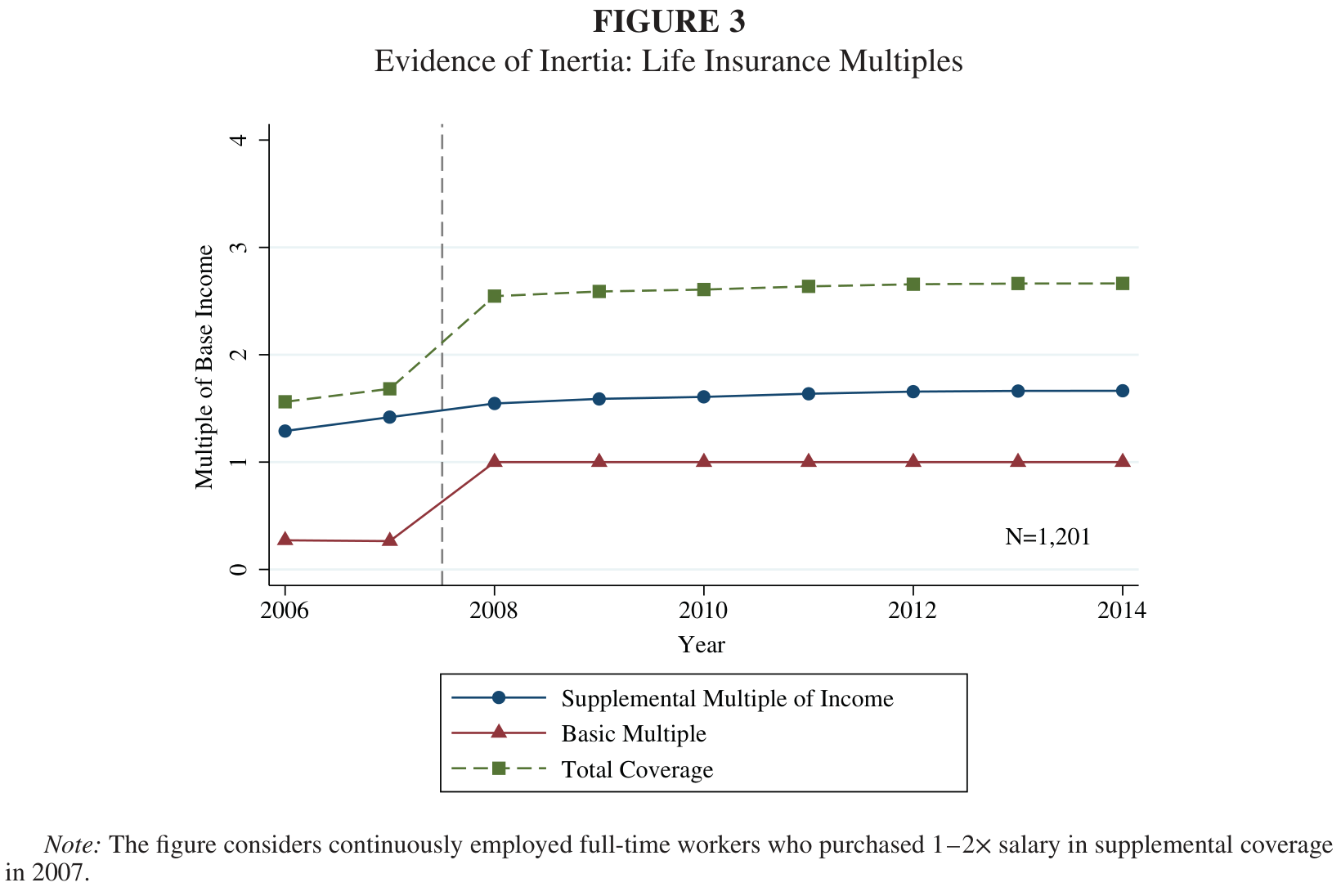
We illustrate the influence of increased basic life insurance in Figure 3 for employees who are at an interior solution in 2007. The figure provides strong evidence of inertia and that the nudge significantly increased total ESLI coverage.

Figure 3. Evidence of Inertia: Life Insurance Multiples

Figure 3. Coverage multiples for 1,201 continuously employed workers, 2006–2014. Basic coverage jumps to one times salary in 2008; supplemental coverage remains near one-and-a-half times salary, so total coverage rises. The vertical dashed line marks the policy change. — Figure 3. Open full-resolution image.

Notes: The figure considers continuously employed full-time workers who purchased 1–2× salary in supplemental coverage in 2007.

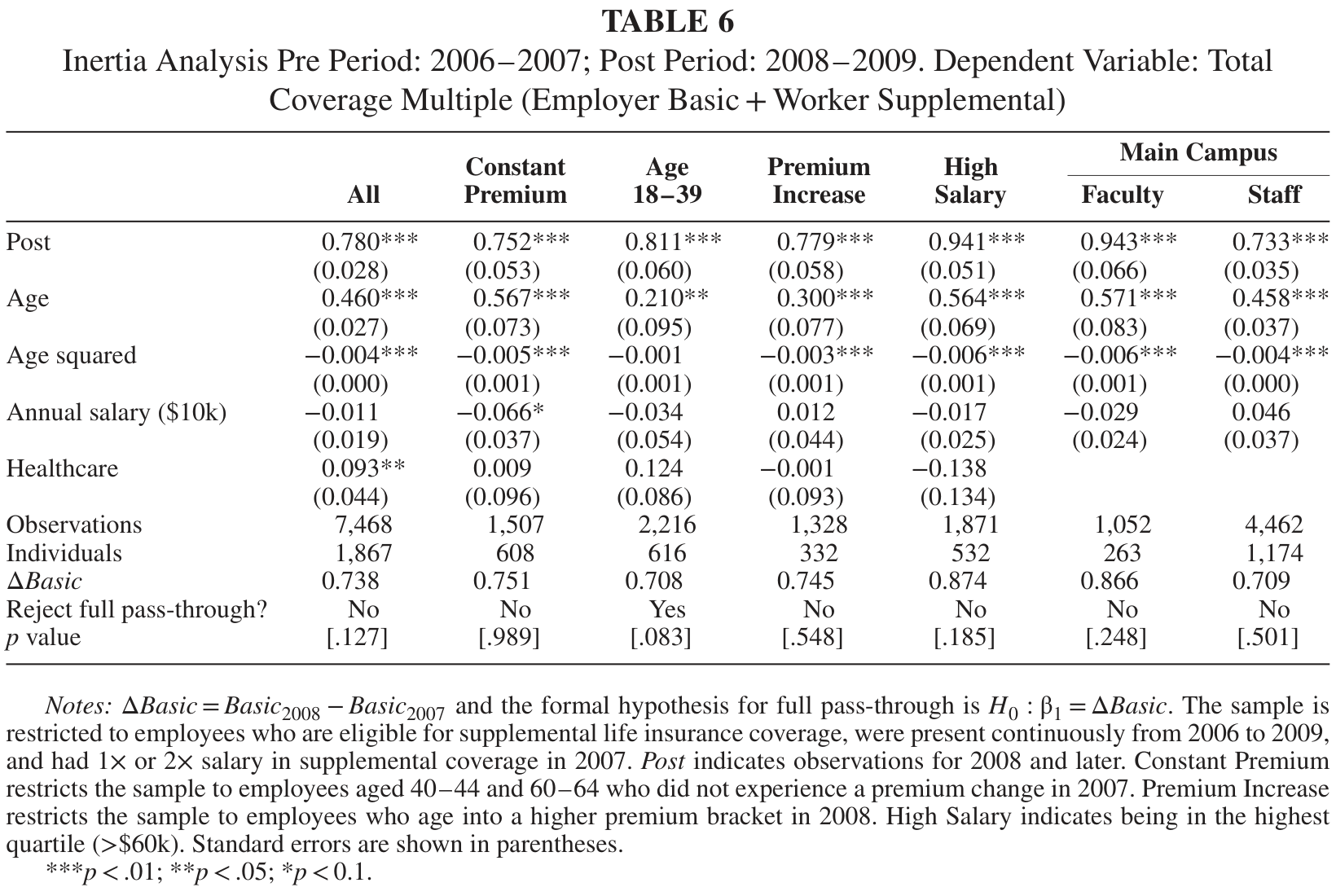
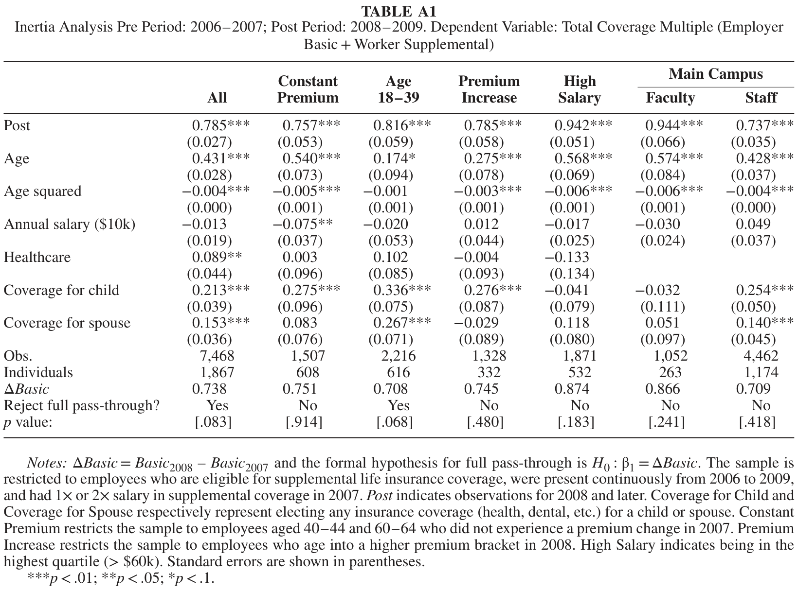
To formally test this finding, we estimate the fixed effect regression given in Equation (2). We use the 2 years on either side of the policy change to capture the short-run effects. In the first column of Table 6, the coefficient on Post Change t indicates that the average increase of 0.74× salary in basic life insurance (from $10,000 to 1× salary) caused an increase in multiple of total coverage (basic + supplemental) of 0.78× salary. We cannot reject the null hypothesis of full pass-through of the increase in basic coverage into total coverage (between 98 and 113% pass-through at the 95% confidence level).²³ This result provides strong evidence that existing employees did not respond to the change in the default level of coverage.

We next consider employees between the ages of 40–44 and 60–64 who did not experience premium changes in 2007 and consequently represent our cleanest sample. This age restriction leads to the same conclusion as the full sample that we cannot reject full pass-through of the increase in basic coverage. We then restrict the sample to include just those individuals aged 18–39 years. As mentioned, these individuals experienced a sizable increase in premiums (50 to 60%) in 2007, 1 year before the change in basic coverage. If employees react the following year to the price increase then this would indicate crowd-out of the increase in basic coverage. The premium change for this age group should exaggerate any crowd-out that we find or equivalently should understate inertia. The third column of Table 6 shows that for a 0.71× salary increase in basic coverage, employees increase total coverage by 0.81× salary. Once again, we conclude full pass-through of the increase in basic coverage even with any influence of the premium increase. In addition, we examine employees that experienced an increase in premium due to aging into a higher premium bracket in 2008 and continue to find full pass-through of the increase in basic coverage.

Table 6. Inertia Analysis Pre Period: 2006–2007; Post Period: 2008–2009. Dependent Variable: Total Coverage Multiple (Employer Basic + Worker Supplemental)

Table 6. Inertia regressions comparing 2006–2007 with 2008–2009 for total basic-plus-supplemental coverage. Seven columns cover the full sample and premium, age, salary, faculty and staff subgroups, with coefficients, standard errors, sample sizes and full-pass-through tests. — Table 6. Open full-resolution image.

High earners experience the largest increase in basic coverage and therefore should be the most likely to decrease supplemental coverage. For example, someone making $30,000 mechanically received $20,000 more basic coverage whereas someone making $100,000 received an additional $90,000 in basic coverage. The fourth column shows that the result of full pass-through holds even when we restrict the analysis to the highest earning quartile. This finding decreases the likelihood that the pass-through is caused by the discrete options of supplemental coverage as high earners should have reacted more relative to low earners. Additionally, we cannot reject the hypothesis of full pass-through when we break out the sample by faculty and main campus staff.

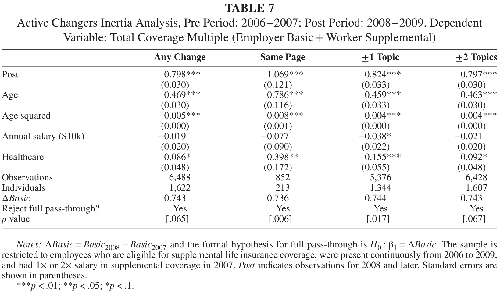
One explanation for these findings is that employees faced prohibitively high time costs, which resulted in employees not reducing coverage in response to the increase in basic coverage. Employees in 2008 needed to submit a paper form to the benefits office to change any elections. However, employees that were already walking to the benefits office to change other elections faced a much lower cost to change supplemental ESLI coverage. The first column of Table 7 restricts the sample to individuals that changed any other election (health, vision, dental, etc.) in 2008 and that elected 1–2× coverage in 2007. Even with reduced time costs, we continue to find full pass-through of the increase in basic coverage.

Another possible explanation for the full pass-through is inattention or ignorance (Choi 2015). If employees were unaware of the increase in basic life insurance coverage, then they would not have reacted to the policy change. To investigate this explanation, we examine employees that changed other portions of their benefit packages in 2008. Individuals who made changes to any election likely consulted the University’s benefits book and were more likely informed about the change in life insurance coverage. A potential concern is that individuals who changed a single election only looked at that specific benefit (i.e., health flexible spending account [FSA]) and did not even notice the change in basic life insurance. To address this, we analyze individuals who make changes to a benefit election located on the same page as life insurance in the benefit book. This increases the likelihood that employees are aware of the change in life insurance. We further expand this by varying the sample based on changing benefits listed in varying proximity to life insurance in the benefits book. Through all of these specifications, we find more than full pass-through of the increase in basic coverage, which provides stronger evidence that the pass-through is not merely a result of unawareness.

Table 7. Active Changers Inertia Analysis, Pre Period: 2006–2007; Post Period: 2008–2009. Dependent Variable: Total Coverage Multiple (Employer Basic + Worker Supplemental)

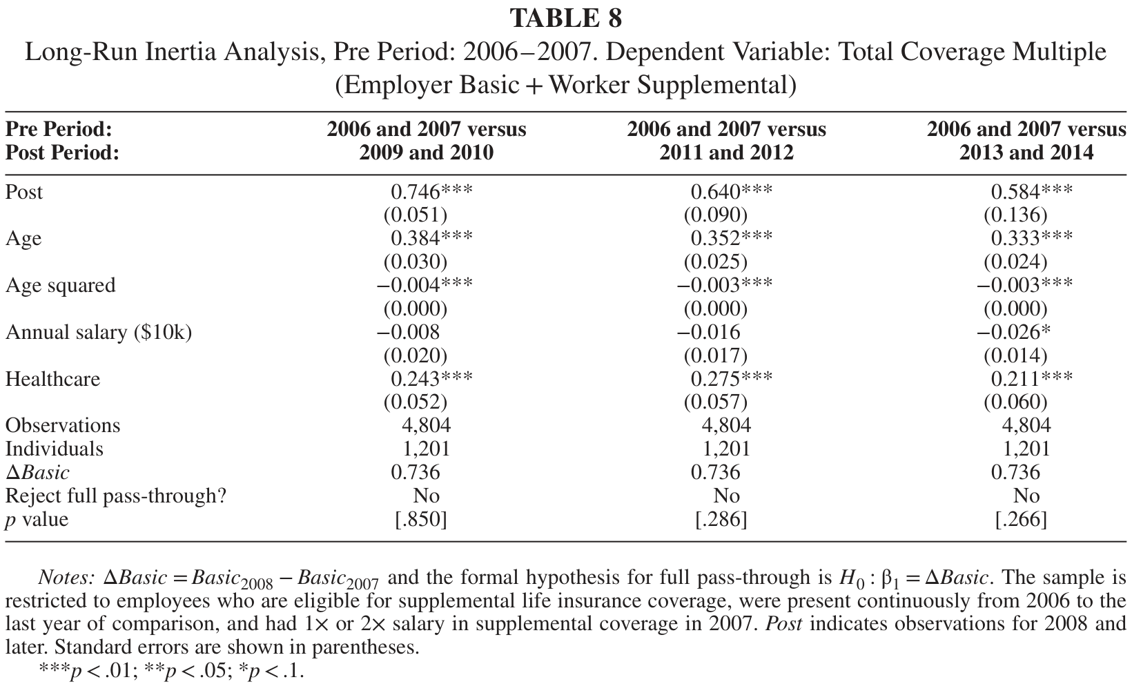
Table 7. Inertia regressions for active benefit changers. Four columns classify any change, same-page change, and changes within one or two topics; rows give coefficients, standard errors, sample sizes and full-pass-through tests for total coverage. — Table 7. Open full-resolution image.

Although in the short run, we find strong evidence of inertia, the increased coverage could be crowded-out over a longer time horizon. In addition, previous studies have mixed results of the persistence of the effects of inertia (Chetty et al. 2014; Jones 2012). Using continuously employed workers from 2006 to 2014, we see how employees initially at the interior (1–2× salary) react. In 2009, the University added the option to make elections online, which should reduce the time costs of changing supplemental coverage and increase the likelihood of crowd-out. The first column of Table 8 gives an estimate for years 2006 and 2007 in comparison to 2009 and 2010 just 2 and 3 years after the change and we fail to reject full pass-through even with the addition of online elections. The second column compares the same pre period with 2011 and 2012 as the post period. The coefficient decreases, in relation to the short-run effect, but we still cannot reject full pass-through. The third column shows that even 6 years after the change, we still cannot reject the hypothesis of full pass-through with a 0.74× salary increase in basic coverage resulting in a 0.58× salary increase in total coverage. Although we cannot reject full pass-through in any of these specifications, the point estimates do decrease over time. This could represent some gradual adjustment or merely a less precise estimator (standard errors significantly increase over time). Additionally, these long-run estimates must be interpreted with caution as many factors likely changed between 2008 and 2014 that could be correlated with demand and preferences for life insurance coverage.

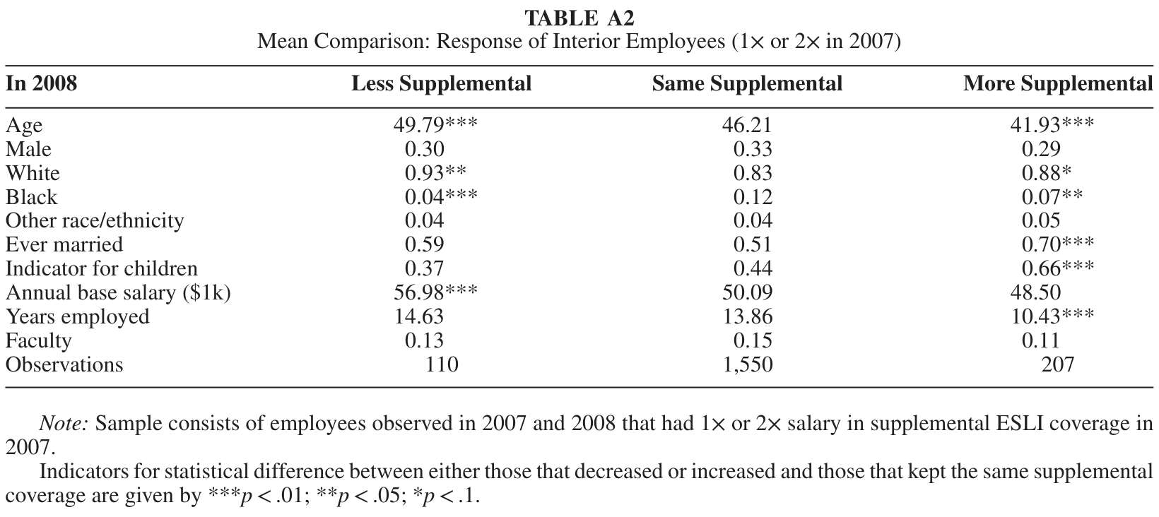
Even though on average, employees do not reduce supplemental coverage in response to the increase in basic coverage there are some employees that increase or decrease coverage. In 2008, 83.0% of employees at the interior (1× or 2×) kept the same level of supplemental coverage as the year before. Only 5.9 decreased coverage and 11.1% increased coverage. Consistent with decreased need and increasing premiums as employees age, older employees (and those that have been employed longer) are more likely to reduce coverage. Additionally, individuals with higher mean earnings are also more likely to reduce supplemental coverage likely due to the correlation with age and years employed. Those with children and spouses are more likely to have increased supplemental coverage consistent with increased demand for replacing foregone salary in the case of death.²⁴

Table 8. Long-Run Inertia Analysis, Pre Period: 2006–2007. Dependent Variable: Total Coverage Multiple (Employer Basic + Worker Supplemental)

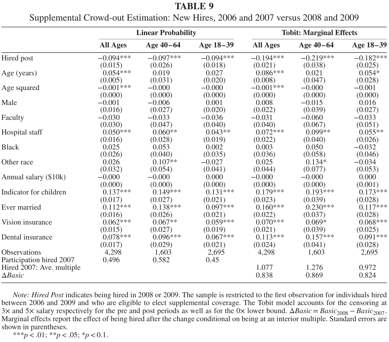
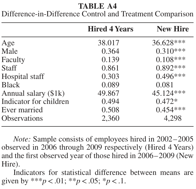
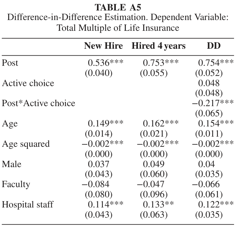
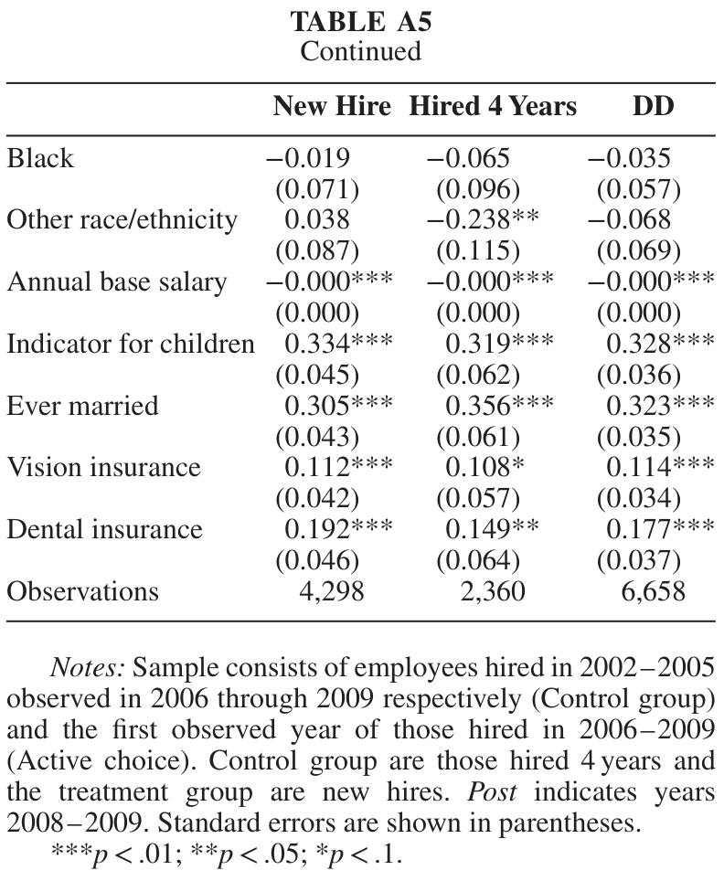
Table 8. Long-run inertia regressions for total coverage: the 2006–2007 baseline is compared with 2009–2010, 2011–2012 and 2013–2014. Coefficients, standard errors, 1,201 individuals, basic-coverage changes and full-pass-through tests are shown. — Table 8. Open full-resolution image.

B. Impact on New Hires: Partial Crowd-Out

Next, we examine the extensive margin (participation in supplemental coverage) for new hires at the University who do not face inertia. We restrict the sample to the first observation for individuals hired between 2006 and 2009.²⁵ The first columns of Table 9 give the linear probability model results from Equation (3) with supplemental participation as the dependent variable. The first column shows that on the extensive margin, individuals hired after the increase in basic coverage are 9.4 percentage points less likely to elect supplemental coverage from a base of 50% participation consistent with the theoretical prediction of crowd-out.²⁶

Those under age 40 experienced increased premiums in 2007—on the order of 50% to 60%—which would bias our results toward finding larger crowd-out effects. We break out the response by ages to address this concern. The same approximate reduction holds for those aged 40 and over who experienced smaller premium changes—ranging from 0 to negative 12%—as well as those under 40.²⁷ Through all specifications, having a child or spouse increases supplemental life insurance participation.

We next estimate a Tobit model to analyze how the change in basic coverage influenced the intensive margin for supplemental coverage. We use a Tobit model to account for individuals who select 0× salary in supplemental coverage and for those that are restricted to purchasing 3× annual salary before the change and 5× annual salary following the change. The latter columns of Table 9 present the marginal effects from Equation (3) with multiple of supplemental coverage as the dependent variable. The coefficient on Hired Post in the fourth column implies that the increase in basic coverage of 0.838× salary caused a multiple reduction of 0.19× salary for those who selected an interior multiple. This implies that for a $100 increase in basic coverage, supplemental coverage was reduced by $23.

The other columns show that this result does not significantly vary across different age groups despite the premium changes in 2007.²⁸ Overall, for new hires—who do not face inertia—the increase in basic coverage caused a decrease in supplemental life insurance participation by 19%. In addition, conditional on electing supplemental coverage, roughly 75% of the increase in basic coverage was passed-through to total ESLI coverage.

Table 9. Supplemental Crowd-out Estimation: New Hires, 2006 and 2007 versus 2008 and 2009

Table 9. Supplemental insurance crowd-out among new hires, comparing 2006/07 with 2008/09. Six columns combine linear-probability estimates and Tobit marginal effects for all ages, ages 40–64 and ages 18–39; controls, sample sizes and model notes are included. — Table 9. Open full-resolution image.

C. Discussion of Results

The results for existing employees in conjunction with the findings of new hires help illustrate the influence of the increase in basic coverage. While we find full pass-through for existing employees, we also find approximately 75% pass-through of the increase in basic coverage for new hires. These findings lead to two important questions. First, what is driving the large pass-through for new hires? Second, what is the explanation for the difference between new hires and existing employees?

The required active choice for new hires precludes inertia as a possible explanation for the first question. A possible explanation for the lack of full crowd-out for new hires is the simultaneous change in available supplemental coverage in 2008. Given the difficulties and uncertainty associated with individual financial planning, the expansion of available multiples from 0–3× to 0–5× salary in addition to the increased maximum face value from $375,000 to $1,000,000 could have induced more coverage. Increased supplemental elections for new hires after 2008 would be consistent with previous findings that individuals tend to choose a middle option to avoid either the minimum or maximum and to compromise between different available choices (Kamenica 2008; Simonson 1989; Simonson and Tversky 1992). In this context, employees might select the middle amount of supplemental coverage to compromise between potentially over- or underinsuring against premature death. This would lead to 2× salary for employees hired prior to 2008 and 3× salary for employees hired in 2008 or later. This behavior is similar to “1/n” savings behavior where investments are influenced by the number of available options (Benartzi and Thaler 2001). It is therefore likely that a portion of the observed pass-through for new hires is due to these context effects.

Another related explanation for the lack of crowd-out is implicit advice. Employees could interpret the increased maximum level of coverage and available multiples as a recommendation for more life insurance coverage. This in turn would counteract part of the crowd-out effect from the increase in basic coverage.

Although these changes occurred for new hires as well as existing employees, previous studies have found that new hires—for whom the policy changes were most salient—respond more to changes in benefit pricing and more frequently elect new options relative to existing employees (Handel 2013; Royalty and Solomon 1999; Samuelson and Zeckhauser 1988; Strombom, Buchmueller, and Feldstein 2002). Additionally, Sheng, Parker, and Nakamoto (2005) find that subjects who are more familiar with a product category (i.e., existing employees) are less likely to select the middle or compromise option. Consequently, in the absence of the change in available supplemental coverage, the crowd-out of the increase in basic coverage for new hires would likely be much greater.

The major difference between new hires and existing employees is the required active choice by new hires. Therefore, the difference between the pass-through of the increase in basic coverage for new hires and existing employees may be attributed to inertia.²⁹ The 25% difference in pass-through—given the context and implicit advice effects described above—represents a lower bound for the influence of inertia on existing employees. Choi (2015) describes many different factors that may contribute to inertia including transaction costs and ignorance. As previously described, the empirical results using changes in other benefit elections indicate that transaction costs and ignorance were likely not the main driving factors of inertia. Nonetheless, the cognitive dissonance associated with thinking about premature death or financial planning could induce inertia. Furthermore, anchoring on the default level of coverage (rather than coverage from the previous year) in conjunction with loss aversion could be contributing to the inertia that we observe. Another likely candidate—given the low probability of premature death and ESLI’s relatively inexpensive nature—is inattention.

An alternative explanation for our finding of full pass-through could be loss aversion. The influence of loss aversion from the discrete nature of supplemental ESLI multiples could describe some of the nonresponse. For example, someone making $40,000 has the choice of $10,000 less ESLI (by decreasing 1× salary) or $30,000 more (by not changing coverage). Additionally, someone making $100,000 would have the choice between $10,000 less or $90,000 more total ESLI. Loss aversion could lead employees to not reduce supplemental coverage in response to the increase in basic coverage. All else equal, it would be expected that loss aversion should influence the lower earner more than the high earner for whom the loss is proportionately small. Nonetheless, we find full pass-through for both high and low earners, which decreases the likelihood that loss aversion is the main cause of the pass-through.³⁰

To summarize, inertia appears to be a contributing factor in the full pass-through of the increase in basic coverage. Presumably, the difference between new hires and existing employees would be larger in the absence of the expansion of available multiples and the maximal face value of supplemental coverage. Therefore, the lower bound for the level of inertia is 25%, but the level of inertia is likely much larger due to implicit advice and context effects that differentially influence new hires.

D. Highly Compensated Employees: Additional Evidence of Inertia

Yet another example of inertia can be found with highly paid employees in 2007 that were constrained at a maximum contribution of $375,000 but that were not constrained by the 3× salary restriction. Individuals who made between $125,000 and $187,500 could not have 3× salary in coverage due to the $375,000 maximum prior to 2008.³¹ For example, an individual who made $160,000 and selected 3× salary would have been assigned a multiple of 2.34 due to the $375,000 limit prior to 2008 despite having picked a whole multiple. The individuals who were constrained by the maximum automatically increased in 2008 to the multiple that they chose previously (in this case 3× salary). Therefore, the policy change not only increased their basic coverage, but also increased their supplemental coverage above what they had (in this example to $640,000 in total coverage).

Among these individuals, many of them presumably had latent demand for more life insurance, which could have been realized following the expansion of the maximum and lead to an election of 4× or 5× salary. Alternatively, they could have satisfied their latent demand for life insurance by purchasing individual market life insurance. In this case, they should decrease supplemental coverage to offset the increased basic life insurance and automatically increased partial multiple of supplemental coverage. Doing nothing in 2008 is an abnormal reaction and indicative of inertia. Of those who were constrained by the $375,000 maximum in 2007 (86 employees), 14% increased to a multiple of 4× or 5× annual salary (latent demand), and 7% reduced their election (crowd-out). The remaining 79% simply allowed a mechanical increase in supplemental coverage to 3× annual salary. Even 3 years after the change over 70% remained at 3× salary in coverage. Although this example deals with a small subset of highly compensated employees, the result still illustrates affluent employees electing life insurance and then not responding to external factors that influence their total coverage. Inasmuch as high compensation implies financial literacy, this result suggests that nonresponse by those at the interior is less likely to be the result of deficiencies in financial understanding.

VI. INDIVIDUAL MARKET CROWD-OUT

The market for life insurance differs from other major forms of insurance (such as health insurance prior to the Affordable Care Act) in that there exists an employer market and a well-functioning individual market. Individual and ESLI differ in that individual policies are experience rated (individually underwritten) and ESLI policies are generally community rated. Additionally, ESLI is conditional on employment whereas term life insurance is merely conditional on premium payments. The experience rating in the individual market also represents an additional cost (time, blood tests, lengthy questionnaires, etc.) in comparison to ESLI costs. Notwithstanding these differences, an individual market term policy is an imperfect substitute for ESLI in terms of actual insurance provided. Therefore, even in the absence of the most natural form of crowd-out (supplemental ESLI), it is possible that employees reduced or lapsed individual market policies as basic ESLI increased.

The University data do not provide information on employees’ individual market life insurance coverage. To understand this relationship, we turn to the SIPP, which has information on holdings from the employer-sponsored market and implicit information on holdings from the individual life insurance market. These data have been used in recent studies on demand for life insurance (Harris and Yelowitz 2014, 2015; Hedengren and Stratmann 2016). This nationally representative longitudinal sample is constructed through individual interviews in 4-month intervals known as waves. Each wave contains responses regarding income, labor force activity, and participation in government assistance programs. In addition to the core monthly questions, the survey covers less-frequently asked subjects in topical modules. The wealth topical modules contain detailed information on assets and liabilities (including life insurance holdings) and are asked at least twice per panel for the survey years used in this analysis. We use SIPP panels from 1996 to 2008 and limit our sample to individuals aged 18–64.³²³³

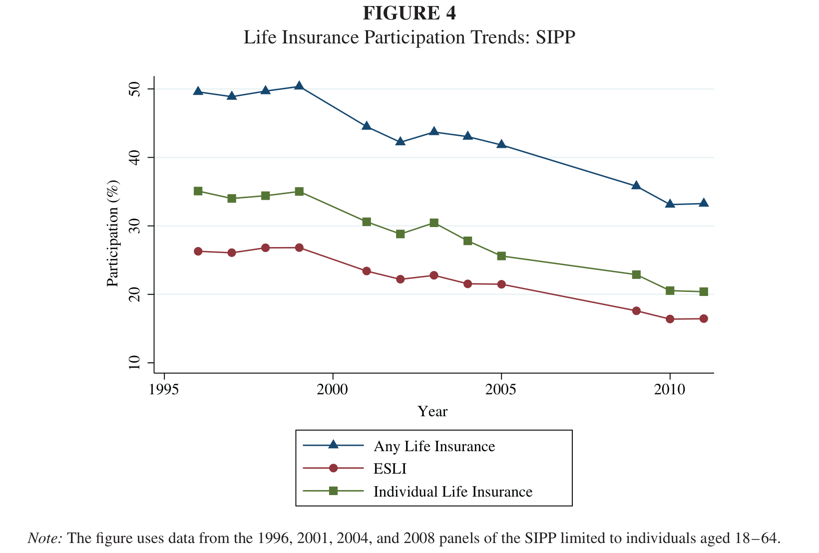
Figure 4. Life Insurance Participation Trends: SIPP

Figure 4. SIPP participation trends from 1996 to 2011. Any life insurance declines from about 50 to 33 percent, individual life insurance from about 35 to 20 percent, and employer-sponsored life insurance from about 26 to 16 percent. Series use distinct markers and a complete legend. — Figure 4. Open full-resolution image.

Note: The figure uses data from the 1996, 2001, 2004, and 2008 panels of the SIPP limited to individuals aged 18–64.

The survey explicitly asks about insurance obtained through an employer and about total life insurance coverage. The difference between total and ESLI holdings allows us to infer individual life insurance holdings.³⁴ Prior to the 2004 panel, the survey asks about the “face value” of policies (the amount that would be paid out at death) which applies to all types of life insurance policies allowing for correct identification of individual life insurance. However, for the 2004 and 2008 panels, the questions changed to asking about the “cash value” of a policy, which only applies to life insurance with an investment portion, primarily whole life insurance. Gottschalck and Moore (2007) show that a majority of respondents did not understand the distinction between cash and face value and continued to report face value even though the question asked cash value. If individuals who only had term life insurance accurately responded to the question following the change, then there would be no way of determining if they had both ESLI and individual life. Consequently, the indicator for individual life insurance is subject to measurement error.

Nonetheless, the SIPP is still the most suitable dataset to explore the relationship between ESLI and individual life insurance. Figure 4 shows that total, ESLI, and individual market life insurance all have decreasing participation over time. Those that held some form of life insurance decreased from 50% to 32% from 1996 to 2011. These declines are consistent with industry-level findings of a 50-year low in life insurance ownership (Prudential 2013). A simple correlation between ESLI and individual life insurance indicates a positive relationship. This could come from the correlation of higher income workers with firms that offer life insurance or represent strong preferences for insurance manifesting itself by having life insurance in both markets. Looking past a simple correlation, we turn to a quasi -experimental approach that examines how job changers react to differences in ESLI offerings from different firms. Employment changes are endogenous, but these changes are arguably orthogonal to changes in life insurance preferences, much like retirement savings (Chetty et al. 2014). ESLI offerings vary tremendously across industry as seen in both the NCS and in the SIPP, yet take-up is very high. For example, in the SIPP, 7% of administrative workers— where duties/quality of the job is thought to be fairly homogeneous—in “employment services” have ESLI, whereas 61% of hospital administrative workers have ESLI.³⁵ Therefore, a change in workplaces could induce an exogenous increase or decrease in ESLI that will be our source of identification for the following fixed effect regression.

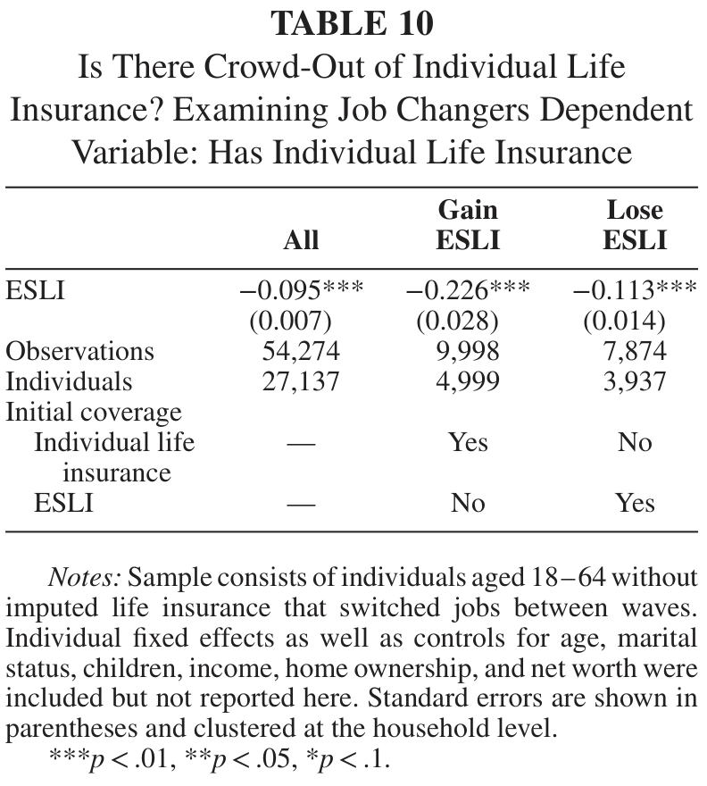
Table 10. Is There Crowd-Out of Individual Life Insurance? Examining Job Changers Dependent Variable: Has Individual Life Insurance

Table 10. Individual-life-insurance crowd-out among job changers: columns show all changers, those gaining employer-sponsored coverage, and those losing it. ESLI coefficients, standard errors, observations, individual counts and initial coverage conditions are reported. — Table 10. Open full-resolution image.

Equation 4. Individual Life for individual i at time t equals delta0 times ESLI i,t plus delta1 times X i,t plus individual effect alpha i and error u i,t. — Equation 4. Open full-resolution image.

{I n d i v i d u a l L i f e}_{i t}

is an indicator for holding individual life insurance, ${E S L I}_{i t}$

is an indicator for employer-sponsored coverage, $X_{i t}$

is a vector of time varying covariates, $α_{i}$

is the individual fixed effect, and $u_{i t}$

is the error term. We restrict our analysis to the year an individual switches employment and the year preceding the change. We only consider changes from one employer to another and only those who do not experience drastic changes in earned income (Chetty et al. 2014).³⁶

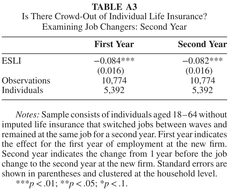
Table 10 shows the results from estimating the model presented in Equation (4). The first column shows that relatively few, 1 in 10, workers have individual market life insurance crowded out by ESLI. This estimate, however, includes individuals who could not adjust the extensive margin for individual life insurance in response to changes in ESLI coverage. In the second column, we restrict the sample to include only those with individual coverage and without ESLI prior to the job change. These individuals were able to reduce individual life insurance coverage in response to receiving ESLI. As expected, we find a larger crowd-out estimate after conditioning on those who could be crowded out with almost 1 in 4 lapsing individual life insurance coverage in response to gaining ESLI. Although there is a significant response for those with individual market coverage, only 30% of workers in the SIPP sample have individual life insurance, which translates into less than 1 in 10 of all employees actually responding. This estimate implies that employers should take into account the proportion of employees with individual life insurance coverage when considering offering or increasing ESLI. To determine how many people would purchase individual market coverage upon lapsing ESLI, we restrict the sample to individuals who had ESLI and did not have individual market coverage in the year prior to changing jobs. As reported in the last column, we find that about 1 in 10 respond to a lapse in ESLI by getting the individual market coverage (conditional on not already having individual life insurance coverage).³⁷

Overall, the above results imply that less than 1 in 10 of all employees would reduce coverage upon receiving ESLI. As discussed above, our sample only includes job changers who should be more responsive in comparison to existing employees. Therefore, the substitution between the individual and ESLI for job changers likely represents an upper bound for the actual level of substitution. In addition, this analysis deals with the extensive margin whereas the policy change at the University only increases the intensive margin, which should elicit less of a response. Hence, we conclude that crowd-out between the group and non-group market is minimal, suggesting that increases in total ESLI coverage represent increases in total life insurance holdings for a majority of employees. This finding of minimal substitution across plans is consistent with findings on retirement savings (Chetty et al. 2014).

VII. DESIRABILITY OF NUDGE

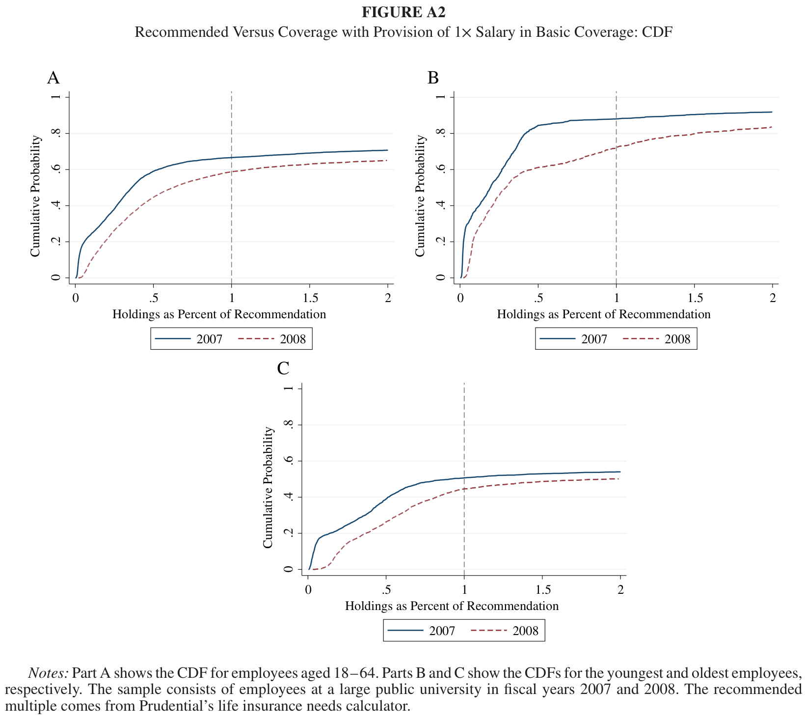
The desirability of the nudge is contingent on the adequacy of employee life insurance holdings. As an approximation, we evaluate employee holdings relative to financial planners’ recommendations. We use a life insurance needs calculator from Prudential to approximate the recommended coverage for each individual. The algorithm uses age, gender, marital status, annual salary, number of children, and age of the youngest child for the recommendation.³⁸

The University data contain information on all these measures with the exception of number of children and age of youngest child. For 52% of the sample, those who do not have children, this limitation is inconsequential. For the portion of the sample with children, we turn to the American Community Survey (ACS) from 2005 to 2013, which has information on number of children and their ages. To obtain a sample of likely employees of the University, we restrict observations to full-time employees of a university or college that reside in the same geographical location as the University. We then impute number of children and age of the youngest child using random draws from the ACS sample conditioned on gender and age bin. With this information, we approximate the recommended amount of coverage for each employee.

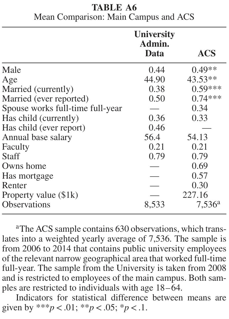
As discussed, our measures for marital status and having children are derived from benefit and insurance elections. Given that individuals might purchase insurance through a spouse, our estimates of recommended coverage are lower than actual recommendations (Ritter 2013). Nonetheless, public employees generally have better employer-sponsored benefits relative to the private sector, which should lessen the bias created by benefits provided through the spouse’s employment (Long and Marquis 1999). As presented in Table A6, only a third of all employees had a spouse that likely had access to employer-sponsored health insurance due to working full-time and full-year. Consequently, the University indicator for marriage does underrepresent actual marriages. However, we see that the indicator for currently having children does not underestimate the measure in the ACS likely due to the relatively generous benefits provided at the University. Notwithstanding, individuals that we classify as being overinsured might have dependents that we do not account for. The bias will result in recommendations that are below what would be the case if we could directly and completely observe family structure.

For employees who could have undone the increase in coverage, 66% had ESLI coverage below the recommended level in 2007. The nudge reduced disparities between ESLI and recommended coverage levels for a majority of these individuals.

The policy variable in this situation is the amount of basic coverage an employer provides, which applies to all employees. Additionally, with the finding of full pass-through, individuals with some supplemental coverage virtually respond the same as those without any supplemental coverage. For these reasons, we evaluate the increase in basic coverage for all employees.

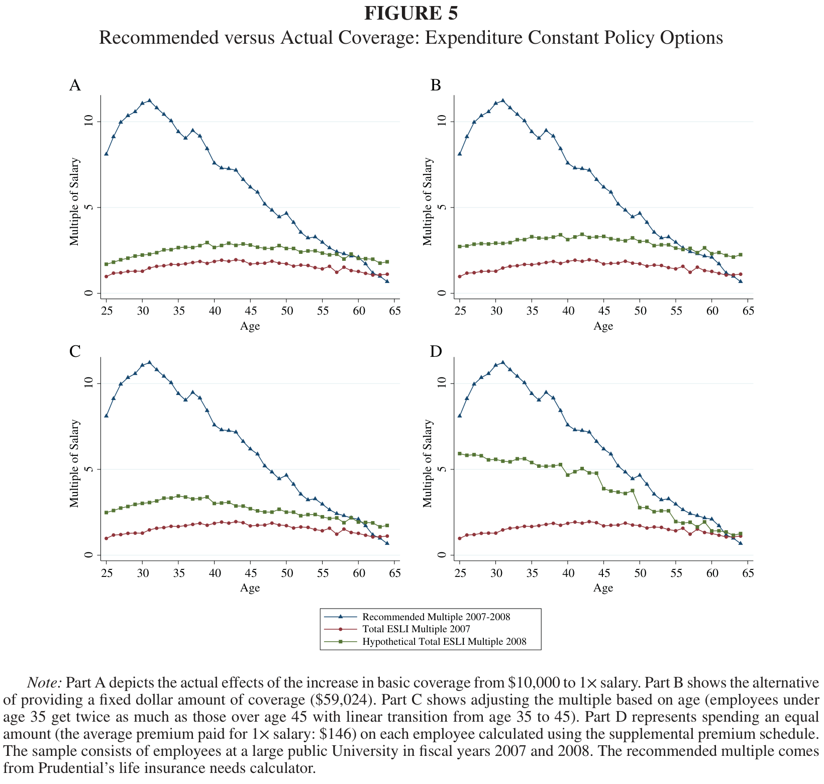
To analyze the effects of the increase in basic coverage, we look at coverage averages from 2007 and 2008 in comparison to the average recommended amount for all employees. Figure 5A shows that the mean multiple of ESLI coverage in 2007 is significantly below the mean recommended multiple for the full sample of employees. The difference between recommended total coverage and actual ESLI coverage is largest for those aged 30–40 and then decreases for older individuals. The increase in basic coverage to 1× salary induced excessive coverage for the oldest employees, but overall it lessened the gap between recommended and actual coverage.

Given that employees do not react to changes in basic coverage, we examine the increase to 1× salary in comparison to alternative expenditure neutral policies targeted at reducing disparities. The disparity between recommended and actual coverage is greater for lower-paid and younger employees. Provision of 1× salary in basic coverage inherently favors those with higher salaries and older employees (where premiums are significantly higher). Hence, uniform provision of a multiple of salary in basic coverage—although the most common form of basic life insurance (57%)—is not the most effective for reducing the average disparity.

Figure 5. Recommended versus Actual Coverage: Expenditure Constant Policy Options

Figure 5. Four expenditure-constant policy comparisons by age: recommended, actual 2007 and hypothetical 2008 life-insurance multiples. Panels compare one-times-salary basic coverage, fixed $59,024 coverage, an age-adjusted multiple, and equal $146 premium spending; the full policy definitions are in the figure note. — Figure 5. Open full-resolution image.

Note: Part A depicts the actual effects of the increase in basic coverage from $10,000 to 1× salary. Part B shows the alternative of providing a fixed dollar amount of coverage ($59,024). Part C shows adjusting the multiple based on age (employees under age 35 get twice as much as those over age 45 with linear transition from age 35 to 45). Part D represents spending an equal amount (the average premium paid for 1× salary: $146) on each employee calculated using the supplemental premium schedule. The sample consists of employees at a large public University in fiscal years 2007 and 2008. The recommended multiple comes from Prudential’s life insurance needs calculator.

An alternative policy, which is used for 38% of workers with basic coverage, is to provide a fixed amount of coverage (keeping total expenditures constant: $59,024) to each employee eliminating the advantage for higher earners (Figure 5B) (LIMRA 2015a). This policy decreases the disparities more relative to 1× salary but still induces excessive coverage for the oldest employees. Inherently, this policy redistributes to lower-paid employees who have larger disparities as measured in multiples of salary. Providing a fixed amount of coverage however, does not address the concern that younger employees generally have larger disparities in coverage.

Another option is to vary the multiple of basic coverage based on age. The Federal Employees’ Group Life Insurance (FEGLI) program is the largest ESLI provider in the United States and uses age-based multiples. Employees 35 and younger get twice the multiple as employees over age 45 with a linear reduction for the 10 years in between. Figure 5C shows how an expenditure neutral application of this policy would affect disparities at the University. As shown, the policy mechanically lessens the gap for younger employees. However, the policy still inherently provides more coverage (in dollars) to higher-paid employees relative to lower-paid employees.

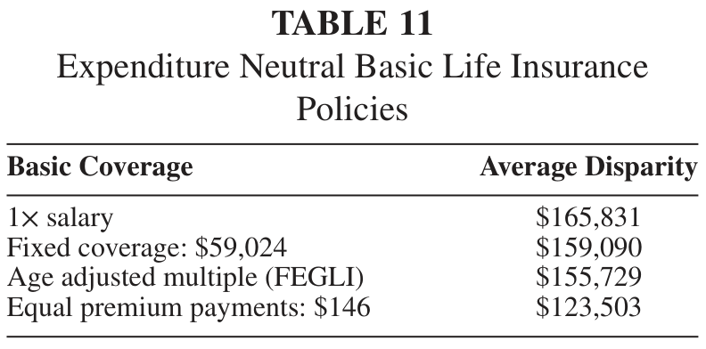
A final policy, which is not commonly used, is to provide equal dollar contributions toward premiums for each employee (keeping total expenditures constant: $146). This policy would not favor the higher-paid employees and would implicitly provide more coverage for the young who face lower premiums. Figure 5D shows that this scenario decreases the disparity between recommended and actual coverage more effectively than a fixed benefit, multiple of salary, or age-adjusted multiple. This finding is consistent with Goda and Manchester (2013) and Handel and Kolstad (2015) who show that varying defaults by observables can increase welfare. In addition, this policy is straightforward to implement and meets legal requirements that prevent discrimination of older employees. Table 11 summarizes the findings by looking at the average disparity under different structures.

Table 11. Expenditure Neutral Basic Life Insurance Policies

Table 11. Average coverage disparity under expenditure-neutral policies: one times salary, $165,831; fixed $59,024 coverage, $159,090; age-adjusted FEGLI multiple, $155,729; equal $146 premium payments, $123,503. — Table 11. Open full-resolution image.

One important qualification with these alternative policy predictions is that they assume the same level of crowd-out as provision of 1× salary, which might not be the case. For example, a 30-year-old employee that makes $30,000 would receive 5× salary in coverage under the equal dollar contribution (rather than 1×) which would likely elicit more crowd-out. Nonetheless, the alternative policies discussed do provide some insight into design for basic coverage to more closely align coverage with recommended levels.

When considering these different alternatives to basic life insurance, we need to consider the incentives faced by employers providing benefits. Even though life insurance is likely not the reason for choosing employment, employers offer life insurance to attract new employees and retain productive ones. A policy such as offering equal contribution toward premiums inherently provides more coverage to younger employees whom an employer might want to attract. Given the nature of ESLI, the oldest employees might experience job lock because retiring means losing life insurance coverage that would be costly in the individual market.

High life insurance coverage for the oldest employees might therefore retain a less productive portion of the work force. Consequently, equal payment of premiums should be attractive to employers not only because it reduces disparities for employees, but also because it potentially attracts new employees and retains productive ones.

If ESLI was the only avenue for obtaining life insurance, we could conclude that the increase in basic coverage in 2008 helped the average employee obtain coverage closer to the recommended level. However, the existence of the individual market makes this conclusion less certain. Based on averages from the SIPP, around 30% of University employees have individual market coverage. If these employees represent workers with the greatest disparities, then the overall disparity in coverage could be much less than Figure 5A illustrates.

Looking at averages ignores heterogeneity in life insurance needs among University employees. In 2007, 33% of employees had more than the recommended amount principally due to not having a spouse or child.³⁹ The increase in basic coverage caused a 7-percentage point increase in employees with more than the recommended amount of coverage. This highlights the major trade-off for the employer of inducing too much coverage for those who either do not need coverage or already have enough and not inducing enough coverage for those that have less than the recommended amount.⁴⁰

Another aspect to consider with provision of basic life insurance is the individual market response. ESLI coverage is inferior to term life insurance because ESLI is conditional on employment whereas term is conditional on premium payments alone. If someone loses their job, they simultaneously lose ESLI coverage. Should employers remove the option of ESLI? Earlier we found that roughly 1 in 10 would purchase individual market coverage in response to a lapse in ESLI. Therefore, even though term life insurance is a more complete form of life insurance, it does not appear that enough people would take up individual coverage in response to an employer forgoing ESLI coverage to increase overall life insurance.

To summarize, there are widespread disparities between actual ESLI coverage and recommended levels with roughly two-thirds of employees below prescribed levels. While the increase in basic coverage to 1× salary lessened disparities, alternative structures—such as equal contributions to premiums—potentially do a better job at reducing the gap. Potential concerns with these findings include not observing individual market coverage, which could lessen disparities, inducing too much coverage for some employees, and crowd-out of supplemental and individual market coverage. Notwithstanding these concerns, it appears that provision of basic coverage can be an important tool for reducing uninsured vulnerabilities.

VIII. CONCLUSION

In 2008, a large public university increased provision of basic life insurance coverage to employees. Contrary to theory, we find full pass-through of the increase in basic life insurance for existing employees with supplemental coverage. In addition, we find significant pass-through for highly compensated employees who were initially constrained by a maximum contribution limit due to inertia. In contrast, new employees, who were forced to make an active decision, decreased supplemental coverage. Therefore, we conclude that inertia is a meaningful factor in the increase in total coverage. Nonetheless, we recognize the possibility of alternative explanations.

Death in the working-age population is a low probability event with catastrophic consequences that can be mitigated through life insurance. However, life insurance ownership is at a 50-year low and research shows uninsured vulnerabilities (Bernheim et al. 2003; Prudential 2013).

Consequently, difficulties arise for many surviving dependents. Using Danish data, Fadlon and Nielsen (2015) find that widows increase their labor force participation by 10–11% to compensate for lost earnings. In addition, McGarry and Schoeni (2005) find high rates of widow poverty in the United States due in part to insufficient life insurance. Our findings shed further light on the potential role of behavioral economics in reducing disparities between recommended and actual levels of life insurance coverage.

We show that the increase in basic life insurance to 1× salary reduced disparities between recommended and actual levels for two-thirds of the University’s employees. Given the lack of significant crowd-out, it appears that many firms with basic coverage below 1× salary could nudge employees to have more coverage without significant employee response. The question remains of how far employers could go before inducing significant crowd-out. Could more ambitious expenditure neutral policies like fixed contributions be effective? The outcome is speculative, but considering our results of high levels of inertia and only partial crowd-out for those who make active decisions, it is likely that such a policy would increase the total coverage.

APPENDIX A: SUPPLEMENTAL INFORMATION AND ROBUSTNESS

Figure A1. University Policy Changes

Figure A1. Reproduction of the university's 2007–08 Life Insurance and AD&D benefits brochure. It announces basic coverage of one times salary from July 1, 2007 and optional coverage of one–five times salary, with underwriting and beneficiary rules. The brochure's own page number is part of the reproduced document. — Figure A1. Open full-resolution image.

Table A1. Inertia Analysis Pre Period: 2006–2007; Post Period: 2008–2009. Dependent Variable: Total Coverage Multiple (Employer Basic + Worker Supplemental)

Table A1. Inertia regressions for total coverage adding child and spouse coverage controls. Seven full-sample and subgroup columns report post-change and demographic coefficients, standard errors, sample sizes and full-pass-through tests for 2006–2009. — Table A1. Open full-resolution image.

Table A2. Mean Comparison: Response of Interior Employees (1× or 2× in 2007)

Table A2. Mean characteristics of workers holding one or two times salary in 2007, grouped by less, unchanged or more supplemental coverage in 2008. Age, demographics, salary, tenure and faculty status are compared; group sizes are 110, 1,550 and 207. — Table A2. Open full-resolution image.

Table A3. Is There Crowd-Out of Individual Life Insurance?

Table A3. Individual-life-insurance crowd-out among job changers in the first and second years: ESLI coefficients −0.084 and −0.082, each with standard error 0.016, based on 10,774 observations and 5,392 individuals. The complete sample note is retained. — Table A3. Open full-resolution image.

APPENDIX B: DIFFERENCE-IN-DIFFERENCE

Table A4. Difference-in-Difference Control and Treatment Comparison

Table A4. Difference-in-differences control and treatment comparison: employees hired four years earlier versus new hires. Rows compare demographics, faculty/staff status, salary, children and marital status, with 2,360 and 4,298 observations and the full sample/significance note. — Table A4. Open full-resolution image.

Table A5. Difference-in-Difference Estimation. Dependent Variable: Total Multiple of Life Insurance

Table A5, first part. Difference-in-differences estimates for total life-insurance multiples: new hires, workers hired four years earlier and the combined DD model. Rows begin with post-change, active-choice and interaction terms, followed by demographic coefficients and standard errors. — Table A5. Open full-resolution image.

Table A5, continued. Remaining race, salary, family and benefit-election coefficients for the new-hire, four-year-hire and DD models. Observations are 4,298, 2,360 and 6,658; complete control/treatment definitions and significance notes follow. — Table A5. Open full-resolution image.

APPENDIX C: ACCURACY OF FAMILY MEASURES

To look at how accurate our measures of marital status and children are, we turn to the American Community Survey (ACS) from 2006–2014. We look at a narrow geographic region that almost surely contains employees of the University. We further restrict the sample to individuals aged 18–64 who work in the industry “EDU-Colleges, Universities, and Professional Schools, Including Junior Colleges,” work full-time (greater than 30 hours per week), work at least 40 weeks out of the year, and are public employees. Given these restrictions, we are very confident that the sample represents employees at the University.

Table A6. Mean Comparison: Main Campus and ACS

Table A6. Mean comparison of university main-campus administrative data and the American Community Survey: demographics, family, salary, faculty/staff status and housing characteristics. The note explains the ACS weighted observations and the two samples' age and employment restrictions. — Table A6. Open full-resolution image.

We compare the ACS sample with full-time University employees in 2008. Given the large number of major hospitals in the region, it is more difficult to pick off likely University employees that worked in healthcare. Consequently, for the comparison we restrict the University sample to main campus employees.

Table A6 shows the comparison between the administrative University data and the ACS sample of likely University employees. Across many dimensions including gender, age, salary, and faculty/staff position, the two samples appear to be very similar. The table shows that the University measure of ever electing spousal coverage underestimates the actual percent of employees that are married. This is partly due to working spouses that have coverage from their employer (Ritter 2013). However, the measure for currently having a child derived from elections seems to closely match the ACS sample. Public employers generally offer better benefits than private employers which makes it more likely that children will be covered through the University employee and consequently be picked up by our metric (Long and Marquis 1999).

APPENDIX D: HETEROGENEITY IN DISPARITIES

As previously illustrated, needs and disparities vary greatly based on age. Figure A2B shows that the increase in basic coverage for employees aged 18–34 caused a 15-percentage point increase in those with at least the recommended level of coverage (from 13% to 28%). The figure also shows a 22% decrease in the number of employees that had less than half of the recommended level (significantly under-insured) and an 8% increase in individuals having more than twice the recommended coverage (over-insured) in part due to not having a dependent. Figure A2C shows that the oldest employees (aged 50–64) were more likely to have at least the recommended level in 2007 (50%). The biggest effect was the 12-percentage point decrease in those that were significantly under-insured. These age differences motivate the potential use of an age adjusted structure rather than a blanket policy such as 1× salary.

Figure A2. Recommended Versus Coverage with Provision of 1× Salary in Basic Coverage: CDF

Figure A2. Cumulative distributions of coverage as a share of recommended coverage in 2007 and 2008: all employees aged 18–64, youngest employees and oldest employees. Each panel shows the 2008 dashed curve below the 2007 curve and marks recommended coverage at a ratio of one. — Figure A2. Open full-resolution image.

Notes: Part A shows the CDF for employees aged 18–64. Parts B and C show the CDFs for the youngest and oldest employees, respectively. The sample consists of employees at a large public university in fiscal years 2007 and 2008. The recommended multiple comes from Prudential’s life insurance needs calculator.

References

Abadie, A., and S. Gay. “The Impact of Presumed Consent Legislation on Cadaveric Organ Donation: A Cross-country Study.” Journal of Health Economics , 25(4), 2006, 599–620.

Ahn, T., and A. Yelowitz. “Paid Sick Leave and Absenteeism: The First Evidence from the U.S.” Working Paper, 2016. Accessed August 2, 2016. http://ssrn.com/abstract=2740366.

Benartzi, S., and R. H. Thaler. “Naive Diversification Strategies in Defined Contribution Saving Plans.” American Economic Review , 91(1), 2001, 79–98.

Bernheim, B. D., L. Forni, J. Gokhale, and L. J. Kotlikoff. “The Mismatch between Life Insurance Holdings and Financial Vulnerabilities: Evidence from the Health and Retirement Study.” American Economic Review , 93(1), 2003, 354–65.

Brown, J. R, and A. Previtero. “Procrastination, Present-Biased Preferences, and Financial Behaviors.” Unpublished Manuscript, University of Illinois at Urbana-Champaign and University of Western Ontario, 2014.

Browne, M. J., and K. Kim. “An International Analysis of Life Insurance Demand.” Journal of Risk and Insurance , 60(4), 1993, 616–34.

Bureau of Labor Statistics, U.S. Department of Labor. “Employee Benefits in the United States, March 2013.” 2013. Accessed November 2015. http://www.bls.gov/ncs/ebs/benefits/2013/ebbl0052.pdf.

Cawley, J., and T. Philipson. “An Empirical Examination of Information Barriers to Trade in Insurance.” American Economic Review , 89(4), 1999, 827–46.

Chetty, R., J. N. Friedman, S. Leth-Petersen, T. H. Nielsen, and T. Olsen. “Active vs. Passive Decisions and Crowd-Out in Retirement Savings Accounts: Evidence from Denmark.” Quarterly Journal of Economics , 129(3), 2014, 1141–219.

Choi, J. “Contributions to Defined Contribution Pension Plans.” Annual Review of Financial Economics , 7, 2015, 161–78.

Choi, J., D. Laibson, and B. C. Madrian. “Mental Accounting in Portfolio Choice: Evidence from a Flypaper Effect.” American Economic Review , 99, 2009, 2085–95.

Choi, J., D. Laibson, B. Madrian, and A. Metrick. “Defined Contribution Pensions: Plan Rules, Participant Decisions, and the Path of Least Resistance.” Tax Policy and the Economy , 16, 2002, 67–114.

———. “For Better or for Worse: Default Effects and 401(k) Savings Behavior,” in Perspectives in the Economics of Aging , edited by D. A. Wise. Chicago: University of Chicago Press, 2004, 81–121.

Conning, Inc. “2014 Life-Annuity Consumer Markets Annual.” 2014. Accessed November 2015. https://www.conning.com/pressrelease-detail.aspx?id=10477.

Dahl, G. B, and S. J. Forbes. “Doctor Switching Costs in Health Insurance.” Working Paper, 2016. Accessed November 2015. http://faculty.weatherhead.case.edu/forbes/Dahl_Forbes_Draft.pdf

Ericson, K. M. M. “Consumer Inertia and Firm Pricing in the Medicare Part D Prescription Drug Insurance Exchange.” American Economic Journal: Economic Policy , 6(1), 2014, 38–64.

Fadlon, I., and T. H. Nielsen. “Household Responses to Severe Health Shocks and the Design of Social Insurance.” Working Paper, 2015. Accessed November 2015. http://www.nber.org/papers/w21352.pdf.

Goda, G. S., and C. F. Manchester. “Incorporating Employee Heterogeneity into Default Rules for Retirement Plan Selection.” Journal of Human Resources , 48(1), 2013, 198–235.

Gottschalck, A. O., and J. C. Moore. “Evaluation of Questionnaire Design Changes on Life Insurance Policy Data Product No. 5, Interagency Agreement (IAA) BC-06-05.” Research Report Series (Survey Methodology #2007–14). Washington, DC: U.S. Census Bureau, 2007.

Gruber, J., and A. Yelowitz. “Public Health Insurance and Private Savings.” Journal of Political Economy , 107(6), 1999, 1249–74.

Handel, B., and J. Kolstad. “Getting the Most from Marketplaces: Smart Policies on Health Insurance Choice.” Brookings Hamilton Project Discussion Paper, 2015.

Handel, B. R. “Adverse Selection and Inertia in Health Insurance Markets: When Nudging Hurts.” American Economic Review , 103(7), 2013, 2643–82.

Harris, T. F., and A. Yelowitz. “Is There Adverse Selection in the Life Insurance Market? Evidence from a Representative Sample of Purchasers.” Economics Letters , 124(3), 2014, 520–22.

Harris, T. F., and A. Yelowitz. “Racial Disparities in Life Insurance Coverage.” Working Paper, 2015. http://ssrn.com/abstract=2600328.

He, D. “The Life Insurance Market: Asymmetric Information Revisited.” Journal of Public Economics , 93(9-10), 2009, 1090–97.

———. “Is There Dynamic Adverse Selection in the Life Insurance Market?” Economics Letters , 112(1), 2011, 113–15.

Hedengren, D., and T. Stratmann. “Is There Adverse Selection in Life Insurance Markets?” Economic Inquiry , 54(1), 2016, 450–63.

Hoynes, H. W., M. D. Hurd, and H. Chand. “Household Wealth of the Elderly under Alternative Imputation Procedures,” in Inquiries in the Economics of Aging , edited by D. A. Wise. Chicago: University of Chicago Press, 1998, 229–57.

Iyengar, S. S., G. Huberman, and W. Jiang. “How Much Choice is Too Much? Contributions to 401 (k) Retirement Plans,” in Pension Design and Structure: New Lessons from Behavioral Finance , edited by O. S. Mitchell and S. P. Utkus. Oxford: Oxford University Press, 2004, 83–95.

Johnson, E. J., and D. G. Goldstein. “Do Defaults Save Lives?” Science , 302, 2003, 1338–39.

Jones, D. “Inertia and Overwithholding: Explaining the Prevalence of Income Tax Refunds.” American Economic Journal: Economic Policy , 4(1), 2012, 158–85.

Kamenica, E. “Contextual Inference in Markets: On the Informational Content of Product Lines.” American Economic Review , 98(5), 2008, 2127–49.

Kopczuk, W., and J. Slemrod. “Denial of Death and Economic Behavior.” Advances in Theoretical Economics , 5(1), 2005, 1–26.

Kotlikoff, L. J., and D. A. Wise. “The Incentive Effects of Private Pension Plans,” in In Issues in Pension Economics , edited by Z. Bodie, J. B. Shoven, and D. A. Wise. Chicago: University of Chicago Press, 1987, 283–340.

Li, D., F. Moshirian, P. Nguyen, and T. Wee. “The Demand for Life Insurance in OECD Countries.” Journal of Risk and Insurance , 74(3), 2007, 637–52.

LIMRA. “Facts of Life: Life Insurance Available through the Workplace.” 2015a. Accessed November 2015. http://www.limra.com/uploadedFiles/limra.com/LIMRA_Root/Posts/PR/_Media/PDFs/2015-LIAM-fact-sheet_Group.pdf.

———. “Life Insurance Coverage Gap Substantial and Growing.” 2015b. Accessed November 2015. http://www.limra.com/Posts/PR/Industry_Trends_Blog/LIMRA__Life_Insurance_Coverage_Gap_Substantial_and_Growing.aspx.

Long, S. H., and S. M. Marquis. “Comparing Employee Health Benefits in the Public and Private Sectors, 1997.” Health Affairs , 18(6), 1999, 183–93.

Lusardi, A., and O. S. Mitchell. “Financial Literacy and Planning: Implications for Retirement Well-Being.” Pension Research Council Working Paper WP2006-01, 2006.

———. “Financial Literacy and Retirement Preparedness: Evidence and Implications for Financial Education.” Business Economics , 42(1), 2007, 35–44.

Madrian, B. C. “Employment-Based Health Insurance and Job Mobility: Is There Evidence of Job-Lock?” Quarterly Journal of Economics , 109(1), 1994, 27–54.

———. “Applying Insights from Behavioral Economics to Policy Design.” Annual Review of Economics , 6(1), 2014, 663–88.

Madrian, B. C., and D. F. Shea. “The Power of Suggestion: Inertia in 401(k) Participation and Savings Behavior.” Quarterly Journal of Economics , 116(4), 2001, 1149–87.

Marton, J., and A. Yelowitz. “Medicaid Auto-Assignment and Participant Inertia.” Working Paper, University of Kentucky, 2016. Accessed August 2, 2016. https://ashecon.confex.com/ashecon/2016/webprogram/Paper3509.html

McGarry, K., and R. F. Schoeni. “Medicare Gaps and Widow Poverty.” Social Security Bulletin , 66(1), 2005, 58–74.

Messacar, D. “The Crowd-Out Effects and Welfare Implications of Retirement Savings Nudges.” Unpublished manuscript, University of Toronto, 2014.

Pauly, M. V., K. H. Withers, K. Subramanian-Viswana, J. Lemaire, and J. C. Hershey. “Price Elasticity of Demand for Term Life Insurance and Adverse Selection.” NBER Working Paper No. 9925. Cambridge, MA: National Bureau of Economic Research, 2003.

Prudential. “The Life Insurance Coverage Gap: Strategies for Financial Professionals to Close the Gap.” 2013. Accessed November 2015. https://www.lifehappens.org/wp-content/uploads/2015/02/Research_TheLifeInsuranceCoverageGap.pdf.

Ritter, J. A. “Racial and Ethnic Differences in Nonwage Compensation.” Industrial Relations: A Journal of Economy and Society , 52(4), 2013, 829–52.

Royalty, A. B., and N. Solomon. “Health Plan Choice: Price Elasticities in a Managed Competition Setting.” Journal of Human Resources , 34(1), 1999, 1–41.

Samuelson, W., and R. Zeckhauser. “Status Quo Bias in Decision Making.” Journal of Risk and Uncertainty , 1(1), 1988, 7–59.

Scism, L. “Struggling Life-Insurance Companies Look to Middle-Class for Revival.” The Wall Street Journal , 2014. Accessed November 2015. http://www.wsj.com/articles/struggling-life-insurance-companies-look-to-middle-class-for-revival-1406255402

Sheng, S., A. M. Parker, and K. Nakamoto. “Understanding the Mechanism and Determinants of Compromise Effects.” Psychology & Marketing , 22(7), 2005, 591–609.

Simonson, I. “Choice Based on Reasons: The Case of Attraction and Compromise Effects.” Journal of Consumer Research , 16(2), 1989, 158–74.

Simonson, I., and A. Tversky. “Choice in Context: Tradeoff Contrast and Extremeness Aversion.” Journal of Marketing Research , 29(3), 1992, 281–95.

Strombom, B. A., T. C. Buchmueller, and P. J. Feldstein. “Switching Costs, Price Sensitivity and Health Plan Choice.” Journal of Health Economics , 21(1), 2002, 89–116.

Thaler, R. H., and C. R. Sunstein. Nudge: Improving Decisions about Health, Wealth, and Happiness . New Haven, CT: Yale University Press, 2008.

Viswanathan, K. S., J. Lemaire, K. Withers, K. Armstrong, A. Baumritter, J. C. Hershey, M. V. Pauly, and D. A. Asch. “Adverse Selection in Term Life Insurance Purchasing Due to the BRCA1/2 Genetic Test and Elastic Demand.” Journal of Risk and Insurance , 74(1), 2007, 65–86.

Notes

1. Lower bound calculated using a 99% confidence interval. The point estimate shows that a 0.74× salary increase in basic coverage resulted in a 0.78× salary increase in total coverage.

2. The results are robust to consideration of actuarially fair premiums.

3. Given the specification of the model, there is no income effect from the increase in basic life insurance even if the employee does not pay the premium. This is the case because inherent to the model is that life insurance is meant to insure against potential lost earnings and not to insure against already received wealth. Any “income effect” would just increase wealth in this model, which is present in both states of the world and therefore irrelevant in the decision of how much life insurance to have. Nonetheless, a model that incorporates more time periods could result in an income effect if provision of basic coverage raised total compensation in later periods.

4. Qualified employees include regular full-time employees or part-time employees ≥.75 full-time equivalent and constitute 91% of all workers.

5. We do not have information on the exact announcement date of the increase in basic life insurance. Nonetheless, it would be atypical for the University to announce the change significantly before the open enrollment period in which it would go into effect. Therefore, there likely were not any anticipatory effects.

6. The University also switched insurance companies in 2008. Both companies have identical and excellent credit ratings. Given the straightforward nature of these life insurance policies, it is unlikely that this switch significantly influenced participation.

7. Prior to 2008, employees were only required to submit a medical evidence of insurability form if they increased supplemental coverage by more than 1× annual salary in a given year. Nonetheless, employees can quickly raise coverage without health screening by increasing supplemental elections by a multiple each year. This requirement should mainly influence the small proportion of employees who received large negative health shocks with imminent mortality (e.g., diagnosis of terminal cancer). Starting in 2008, employees who elected more than $375,000 in supplemental coverage were required to submit a medical evidence of insurability form. This restriction only potentially applies to 14% of employees (those who made more than $75,000). New hires after 2008 could elect 0–3× salary in supplemental coverage without proof of insurability, but were required to submit the form if they initially elected 4× or 5× salary. Nonetheless, new hires desiring more coverage can increase to the maximum level of coverage within 2 years without proof of insurability (conditional on not exceeding $375,000).

8. Previous studies have estimated the price elasticity of demand for term life insurance to be between −0.30 and − 0.66 (Pauly et al. 2003; Viswanathan et al. 2007).

9. An employee gets $375,000 in supplemental coverage if their selected multiple would cause coverage to exceed the maximum. For example, an employee with a base salary of $200,000 who selected 2× salary in supplemental coverage would be assigned a multiple of 1.875× salary due to the $375,000 maximum. Consequently, highly compensated employees (salary $> $ 125, 000$ ) could have a “partial” multiple of supplemental coverage prior to 2008.

10. For a majority of employees examined in this study, the election of supplemental coverage was chosen before 2006 under a framework where employees elected a total multiple of coverage (1×, 2×, and 3× salary) rather than the current system of electing supplemental multiples to be added to basic coverage. It is unlikely that a significant amount of employees lowered supplemental coverage due to the slight increase in total coverage in 2006. Therefore, by revealed preference, a majority of employees preferred the lower multiple rather than the higher multiple that resulted due to the increase in basic coverage.

11. The income elasticity of life insurance coverage has been estimated to be between 0.32 and 0.6, which translates into a negligible increase in life insurance coverage due to the slight increase in total compensation (Browne and Kim 1993; Li et al. 2007). For example, a 35-year-old employee making $50,000 with 1× salary in supplemental coverage would increase coverage to $50,026 as a result of the income effect using an income elasticity of 0.6. Therefore, it is unlikely that any nonresponse originates from an income effect.

12. It is possible that corner constrained individuals had preferences such that $V (4 x) > V (3 x + $ 10 k)$ and $V (4 x) > V (5 x)$ salary such that it was not optimal to increase or decrease supplemental coverage.

13. For the University, fiscal years go from July to June. For example, fiscal year 2006 begins July 1, 2005 and ends June 30, 2006.

14. The open enrollment period is approximately 30 days from mid-April to mid-May. In the case of a qualifying event, all changes must be made within 30 days of the event.

15. If the employee chooses to leave the University, the worker does have the option of switching the policy over to the insurer without health screening. However, according to a Human Resource representative, the worker will “pay dearly” in premiums for the policy. This is referred to as “portability” in the insurance contract. This university is far less explicit than some others with respect to job-related leaves and portability, but appears very similar. If a worker qualifies for LTD, the life insurance policy will end upon turning age 67.

16. We do not observe marital status or children directly in the data. The variables are determined based on health, dental, vision, and dependent life insurance elections as well as dependent flexible spending account (FSA). If an employee ever elects either spousal or family insurance (of any type), then the individual is categorized as “Married in Sample.” Similarly, if an employee elects child or family insurance (of any type) or uses a dependent FSA then they are classified as having a “Child in Sample.” This measure will not pick up individuals who have alternative sources of insurance such as a spouse’s employer (Ritter 2013). In addition, this variable will miss individuals with children who are no longer dependents.

17. Even though we do not explicitly observe education, the position of faculty or staff at the main campus is correlated with level of education (Brown and Previtero 2014).

18. Note that most of the employees are staff and a majority of new hires in 2008 and 2009 were made for the healthcare portion of the University. This is important because both staff and hospital personnel do not necessarily follow the same hiring patterns as faculty.

19. If the University did change the policy to reflect demand for more coverage, it is unlikely that the demand came from the subsample of employees without the maximum supplemental coverage that we focus on in this analysis.

20. This sample additionally excludes those who elected 2× salary in 2007 and had a salary greater than $125,000 and those who elected 1× salary who had a salary greater than $187,500 because they were potentially constrained by the maximum coverage limit of $375,000. In addition, this restriction avoids any conflict with the medical evidence of insurability needed for coverage greater than $375,000. This exclusion represents 1% of those at the interior.

21. One potential limitation of the specification is that it does not account for changes in the employees’ personal circumstances that might influence demand. Nonetheless, this will only bias our results inasmuch as changes in personal circumstances are correlated with the increase in basic coverage, which is likely not the case. The results presented are robust to including annual measures for electing any coverage (health, dental, vision, etc.) for a spouse/child that should reflect changes in family structure or spousal employment (see Appendix Table A1).

22. Employees must select “Basic Life Only” or “Basic Life & Optional Life = [Multiple] × salary” when they are initially hired.

23. Equivalently, we cannot reject the hypothesis of no response from employees.

24. Appendix Table A2 provides a mean comparison for employees that decreased coverage, kept the same coverage, or increased supplemental coverage in 2008.

25. We use the first observation because individuals hired during the fiscal year do not appear in the data until the following fiscal year.

26. Nearest neighbor matching analysis indicates a statistically significant 9.2-percentage point decrease in supplemental coverage for those hired after the increase in basic coverage comparable to the linear probability results.

27. For new hires aged 40 and over, this specification could understate the existence of crowd-out due to the slight (0–12%) decrease in premiums.

28. Similar results were found using a difference-in-difference framework presented in the Appendix. Additionally, Ordered Probit estimates have consistent qualitative results showing that the increase in basic coverage decreased supplemental coverage for new hires.

29. Another possible explanation is optimal nonresponse. However, the small proportion of employees for whom it was not optimal to respond to the policy change with a lower level of supplemental coverage is likely similar for new hires and existing employees. Therefore, optimal nonresponse might explain part of the pass-through of the increase in basic coverage for both new hires and existing employees, but it likely does not explain the difference between the two groups.

30. Yet another explanation for the full pass-through could be a flypaper effect where employees do not take into account employer contributions when electing ESLI. However, if it were just a flypaper effect, we should not observe a difference in pass-through of basic ESLI between new hires and existing employees.

31. In addition, those that made between $187,500 and $375,000 would only have coverage of less than 2× salary. However, this group could have elected either 2× or 3× salary and either way be constrained by the $375,000 maximum.

32. Following Gruber and Yelowitz (1999), we exclude imputed values for life insurance due to criticism of the SIPP wealth imputation methodology by researchers (Hoynes, Hurd, and Chand 1998).

33. Earlier panels of the SIPP do not allow repeat observations of ESLI and individual market elections. Our identification strategy relies on following individual life insurance elections across time which precludes their use.

34. We exclude observations where top coding makes individual life insurance holdings indeterminate, which constitute 0.52% of the sample.

35. See Ahn and Yelowitz (2016) for an example of this type of analysis on paid sick leave.

36. We define a job change based on a change in employer ID and a start date between periods or a change in occupation code. We limit the sample to employees who experienced a change in income from 50% to 150% of previous income.

37. Appendix Table A3 shows that crowd-out from 1 year is roughly equivalent to the crowd-out after 2 years. This does not rule out the possibility of future lagged crowd-out effects, but it does suggest that the cumulative crowd-out is likely not significantly different from the initial crowd-out.

38. The calculator uses data from the Federal Reserve 2010 Survey of Consumer Finances, College Board, 2012 Bureau of Labor Statistics NAHB Survey, Current Population Survey Annual Social and Economic Supplement, and the Consumer Expenditure Survey to calibrate the model. Estimated needs appear to reflect the principal purpose for life insurance of replacing the lost earnings of a breadwinner. For example, needs decrease as an individual approaches retirement. Nonetheless, Prudential sells life insurance and may have the incentive to overestimate needs. The website explicitly states that the amount given should be a starting point for estimating needs. See https://isso.prudential.com/simplifiedneeds/life for documentation on the needs calculator.

39. It is likely that a portion of those we classify as overinsured are classified as such due to our imprecise measures of family structure rather than exceeding the recommended level of coverage.

40. In Appendix C, we look at the effects of the increase in basic coverage on the distribution of disparities for all employees and by age groups.

Abstract

Recommended citation

Related materials

Full article

Abstract

I. INTRODUCTION

Abbreviations

II. POLICY CHANGES AND THEORETICAL PREDICTIONS

Table 1. Employer-Sponsored Life Insurance Policy Details

Figure 1. Interior Solution

III. DATA

A. Description

Table 2. Summary Statistics and ESLI Participation: University Data; Numbers in Percent Unless Denoted

Figure 2. Supplemental ESLI Participation: University Data

B. Representativeness

Table 3. University Comparison, Maximum Effective Multiple

Table 4. National Compensation Survey 2013, ESLI

IV. EMPIRICAL STRATEGY

A. Existing Employees at the Interior

B. New Hires

Table 5. New Hire Mean Comparison University Data; Numbers in Percent Unless Denoted Otherwise

V. RESULTS

A. Impact on Existing Employees: Complete Pass-Through

Figure 3. Evidence of Inertia: Life Insurance Multiples

Table 6. Inertia Analysis Pre Period: 2006–2007; Post Period: 2008–2009. Dependent Variable: Total Coverage Multiple (Employer Basic + Worker Supplemental)

Table 7. Active Changers Inertia Analysis, Pre Period: 2006–2007; Post Period: 2008–2009. Dependent Variable: Total Coverage Multiple (Employer Basic + Worker Supplemental)

Table 8. Long-Run Inertia Analysis, Pre Period: 2006–2007. Dependent Variable: Total Coverage Multiple (Employer Basic + Worker Supplemental)

B. Impact on New Hires: Partial Crowd-Out

Table 9. Supplemental Crowd-out Estimation: New Hires, 2006 and 2007 versus 2008 and 2009

C. Discussion of Results

D. Highly Compensated Employees: Additional Evidence of Inertia

VI. INDIVIDUAL MARKET CROWD-OUT

Figure 4. Life Insurance Participation Trends: SIPP

Table 10. Is There Crowd-Out of Individual Life Insurance? Examining Job Changers Dependent Variable: Has Individual Life Insurance

VII. DESIRABILITY OF NUDGE

Figure 5. Recommended versus Actual Coverage: Expenditure Constant Policy Options

Table 11. Expenditure Neutral Basic Life Insurance Policies

VIII. CONCLUSION

APPENDIX A: SUPPLEMENTAL INFORMATION AND ROBUSTNESS

Figure A1. University Policy Changes

Table A1. Inertia Analysis Pre Period: 2006–2007; Post Period: 2008–2009. Dependent Variable: Total Coverage Multiple (Employer Basic + Worker Supplemental)

Table A2. Mean Comparison: Response of Interior Employees (1× or 2× in 2007)

Table A3. Is There Crowd-Out of Individual Life Insurance?

APPENDIX B: DIFFERENCE-IN-DIFFERENCE

Table A4. Difference-in-Difference Control and Treatment Comparison

Table A5. Difference-in-Difference Estimation. Dependent Variable: Total Multiple of Life Insurance

APPENDIX C: ACCURACY OF FAMILY MEASURES

Table A6. Mean Comparison: Main Campus and ACS

APPENDIX D: HETEROGENEITY IN DISPARITIES

Figure A2. Recommended Versus Coverage with Provision of 1× Salary in Basic Coverage: CDF

References

Notes