Early Impacts of the Affordable Care Act on Health Insurance Coverage in Medicaid Expansion and Non-Expansion States

Authors: Charles Courtemanche, James Marton, Benjamin Ukert, Aaron Yelowitz, and Daniela Zapata
Citation: Charles Courtemanche, James Marton, Benjamin Ukert, Aaron Yelowitz, and Daniela Zapata (2017). Early Impacts of the Affordable Care Act on Health Insurance Coverage in Medicaid Expansion and Non-Expansion States. Journal of Policy Analysis and Management 36(1): 178–210. DOI: 10.1002/pam.21961.

© 2016 by the Association for Public Policy Analysis and Management. Published by Wiley Periodicals, Inc.

Abstract

The Affordable Care Act (ACA) aimed to achieve nearly universal health insurance coverage in the United States through a combination of insurance market reforms, mandates, subsidies, health insurance exchanges, and Medicaid expansions, most of which took effect in 2014. This paper estimates the causal effects of the ACA on health insurance coverage in 2014 using data from the American Community Survey. We utilize difference-in-difference-in-differences models that exploit cross-sectional variation in the intensity of treatment arising from state participation in the Medicaid expansion and local area pre-ACA uninsured rates. This strategy allows us to identify the effects of the ACA in both Medicaid expansion and non-expansion states. Our preferred specification suggests that, at the average pre-treatment uninsured rate, the full ACA increased the proportion of residents with insurance by 5.9 percentage points compared to 2.8 percentage points in states that did not expand Medicaid. Private insurance expansions from the ACA were due to increases in both employer-provided and non-group coverage. The coverage gains from the full ACA were largest for those without a college degree, non-whites, young adults, unmarried individuals, and those without children in the home. We find no evidence that the Medicaid expansion crowded out private coverage.

INTRODUCTION

The goal of the Patient Protection and Affordable Care Act (ACA) of March 2010 was to achieve nearly universal health insurance coverage in the United States through a combination of insurance market reforms, mandates, subsidies, health insurance exchanges, and Medicaid expansions (Gruber, 2011). These major components of the ACA all took effect in 2014, with the Medicaid expansion being optional for states after a Supreme Court decision. This paper uses data from the American Community Survey (ACS) to evaluate the first-year impacts of the ACA on health insurance coverage levels and sources in both states that expanded Medicaid and those that did not.

The first component of the ACA’s “three-legged stool” involves reforms designed to improve the functioning of the non-group insurance market for consumers who did not have access to employer-provided or public coverage (Gruber, 2011). Insurance market regulations implemented in 2014 such as community rating, guaranteed issue, and minimum coverage requirements aim to ensure the availability of adequate insurance for those with pre-existing conditions. The law also established a Health Insurance Marketplace, commonly referred to as the “Federal Exchange,” to facilitate insurance purchases for individuals and small businesses and stimulate competition among insurance plans. Each state was given the option of establishing their own insurance exchange and 15 states did so in 2014 (Kaiser Family Foundation [KFF], 2014).

These reforms alone would likely lead to an adverse selection death spiral, as an influx of high-cost beneficiaries would drive up premiums for those remaining in the insurance pool (Gruber, 2011). This concern motivated the second leg of the three-legged school: the individual mandate.¹ Beginning in 2014, individuals deemed to be able to afford coverage but electing to remain uncovered were penalized. The penalty varies with income but can reach as high as the total annual premium for the national average price of a Bronze exchange plan.²

Mandating insurance coverage leads to concerns about affordability, which the third leg of the three-legged stool aims to address through subsidies and Medicaid expansions. Sliding scale subsidies in the form of tax credits are available to consumers in every state with incomes between 100 and 400 percent of the Federal Poverty Line (FPL) who do not qualify for other affordable coverage, such as Medicaid. In states that opted to expand Medicaid via the ACA, Medicaid is available up to 138 percent of the FPL with subsidies available for those between 138 and 400 percent of the FPL. In contrast, in non-expansion states Medicaid is only available to those at much lower income levels, particularly for adults without dependent children, with subsidies available for those between 100 and 400 percent of the FPL.³ Previously, Medicaid eligibility was typically tied to those with low income among specific groups, such as children, low-income parents, pregnant women, the disabled, and the elderly. This suggests a major expansion of Medicaid eligibility via the ACA for low-income childless adults.

We estimate the effects of the ACA both with and without the Medicaid expansion using a difference-in-difference-in-differences (DDD) model with the differences coming from time, state Medicaid expansion status, and local area pre-treatment uninsured rates. This last source of variation, which arises because universal coverage initiatives provide the most intense treatments in areas with high baseline uninsured rates, allows us to disentangle the causal effect of the ACA from the underlying time trend while also accounting for the possible endogeneity of state Medicaid expansion decisions. Finkelstein (2007) uses a similar “bite” strategy to identify the impact of Medicare on health care spending. Miller (2012) also uses this approach to estimate the impact of the Massachusetts reform on emergency room utilization without control states.

The ACS is well suited for our study for several reasons. First, it includes multiple categories of health insurance coverage, allowing for an examination of how the ACA affected both private and public coverage (e.g., via exchanges and Medicaid expansions). In addition, with approximately 3,000,000 observations per year and relatively narrow geographic identifiers, the ACS is large enough to precisely estimate the effects for states and many localities. Finally, the ACS is a mandatory survey, reducing concerns about sample selection amongst respondents.

In our full-sample regressions, we estimate that the ACA including the Medicaid expansion increased insurance coverage by 5.9 percentage points at the sample mean pre-treatment uninsured rate, with the effect reaching as high as 15.3 percentage points in the area with the largest uninsured rate. The effect of the ACA without the Medicaid expansion was only 2.8 percentage points at the mean uninsured rate, reaching as high as 7.3 percentage points. Coverage gains in non-Medicaid expansion states came entirely from private insurance, split between employer-provided and non-group coverage. Gains from the Medicaid expansion are exclusively attributable to increased Medicaid coverage, and we find no evidence of crowd-out of private coverage. These results all remain similar across a wide range of robustness checks and pass falsification tests for differential pre-treatment trends. Subsample analyses show that the increases in coverage from the full ACA were largest for those without a college degree, non-whites, 19- to 34-year-olds, unmarried individuals, and those without children in the home.

LITERATURE REVIEW

There is an extensive literature examining the impact of policies designed to increase insurance coverage on the receipt of both public and private insurance coverage. Buchmueller, Ham, and Shore-Sheppard (2015) provide a thorough review of studies on the impact of expansions of the Medicaid program over time as well as other Medicaid policy changes that may impact coverage.⁴ A recent state coverage expansion that has received a great deal of attention is the Massachusetts insurance market reform of 2006. Using a similar combination of policies to the ACA, the Massachusetts law decreased the state’s uninsured rate by around 6 percentage points (Courtemanche & Zapata, 2014; Long, Stockley, & Yemane, 2009).

A few studies have reported changes in insurance coverage from before to after the 2014 components of the ACA took effect. Long et al. (2014) compare coverage rates in September 2013 to September 2014 and find an overall increase in coverage of 5.3 percentage points among nonelderly adults using data from the Urban Institute Health Reform Monitoring Survey. Within Medicaid expansion states, they estimate the increase in coverage to be 5.8 percentage points, compared to 4.8 percentage points in non-expansion states. Smith and Medalia (2015) use the Current Population Survey Annual Social and Economic Supplement (CPS) to examine changes in insurance coverage for everyone in the United States, including both children and the elderly. They estimate an overall 2.9 percentage point increase in coverage, which is a combination of a 3.4 percentage point increase in expansion states and a 2.3 percentage point increase in non-expansion states. Courtemanche, Marton, and Yelowitz (2016) find a similar 2.8 percentage point increase in coverage nationally across all ages using data from the ACS.⁵

A major limitation of these descriptive studies is that, since insurance coverage rates fluctuate over time, the extent to which their estimates reflect causal effects of the ACA as opposed to other factors is unclear. For instance, the unemployment rate dropped from 8 to 5.6 percent between the start of 2013 and the end of 2014.⁶

Since employment and health insurance coverage are closely related, we might have expected increases in employer-provided and overall coverage in 2014 even without the ACA. Other confounding factors might include demographic shifts and the underlying upward trend in health insurance premiums.

Two studies, Kaestner et al. (2015) and Wherry and Miller (2016), have sought to identify the causal effect of the ACA’s Medicaid expansion on insurance coverage.⁷ Both studies utilize difference-in-difference methods and a sample of low-socioeconomic-status individuals.⁸ Among a sample of individuals with no further than a high school education from the ACS and CPS, Kaestner et al. (2015) find that the Medicaid expansion increased Medicaid coverage by approximately 4 percentage points and decreased the proportion uninsured by approximately 3 percentage points in 2014. Wherry and Miller (2016) restrict their sample to those in the National Health Interview Survey with family income below 138 percent of the FPL and find that the Medicaid expansion increased Medicaid coverage by 11 percentage points and reduced the uninsured rate by 7 percentage points among this group in the second half of 2014.

Our paper offers several contributions relative to both Kaestner et al. (2015) and Wherry and Miller (2016). First, both papers only develop a causal framework for the Medicaid expansion portion of the ACA and consequently focus only on a low-socioeconomic-status subsample. In contrast, we utilize the full sample of non-elderly adults and develop an identification strategy designed to estimate the causal effect of not only the Medicaid expansion but also the law’s private portion (combination of insurance market reforms, exchanges, mandates, and subsidies). This means we are also the first to estimate the overall causal effect of the fully implemented ACA as well as what share of the coverage gains can be attributed to the private versus Medicaid components.⁹ Next, our triple-difference approach offers an alternative identification strategy for the Medicaid expansion effect that relies on weaker assumptions than a difference-in-differences (DD) model. Specifically, we do not need to assume that Medicaid expansion and non-expansion states shared common counterfactual trends; we instead only need to assume that, to whatever extent such differential trends exist, the difference is not correlated with pre-treatment uninsured rates. Third, while both papers consider only two types of coverage—Medicaid and private—we further distinguish whether the gains in private coverage were from employer-provided or non-group insurance coverage. Finally, we consider heterogeneity along new dimensions, as neither paper stratifies their sample by gender or race.

In a new working paper released shortly after the initial version of our paper, Frean, Gruber, and Sommers (2016) attempt to assess the relative contribution of three components of the ACA in 2014—subsidized premiums for Marketplace coverage, the individual mandate, and the Medicaid expansion—using data from the ACS on non-elderly adults. To identify the effect of the Medicaid expansion, the authors use both variation in the state decisions to expand Medicaid and differential impacts of these decisions across income and family structure, which varied across states since they had different eligibility rules prior to the ACA. The identifying variation for the effect of premium subsidies comes from differences in the effective subsidy rate across income groups and local areas. The variation identifying the effect of the individual mandate comes from differences in the tax penalty across the income distribution.

We view this paper as complementary to our work. Whereas Frean, Gruber, and Sommers (2016) broaden their focus beyond just the Medicaid expansion to also consider the impact of Marketplace subsidies and the individual mandate, we estimate the aggregate impact of all 2014 elements of the ACA using a completely different identification strategy. Thus, our estimates capture aspects of the ACA described in Frean, Gruber, and Sommers (2016) as unmeasured, including the “social effects of the individual mandate” and “simplification of purchasing coverage due to the creation of the marketplaces.” They estimate that the combined impact of their three ACA policies of interest is a 2.3 percentage point increase in coverage, of which roughly 60 percent can be attributed to the Medicaid expansion, 40 percent to the premium subsidies, and essentially none to the individual mandate. We find a larger coverage gain (6 percentage points) from the full ACA and a roughly even split between coverage increases due to the Medicaid and non-Medicaid components.

DATA

Our primary data source is the ACS, a nationwide survey administered by the Census Bureau asking detailed questions about population and housing characteristics. The ACS samples approximately 1 percent of the U.S. population. Like the decennial Census, participation is mandatory, and the survey can be completed online or by mailing in a paper questionnaire. The ACS identifies all 50 states and the District of Columbia, and additionally identifies localities known as Public Use Microdata Areas (PUMAs)—approximately 2,300 areas of at least 100,000 people nested entirely within a state.

The ACS is appealing for our study because its large number of observations, over 3,000,000 individuals per year, allows us to precisely estimate the effects of different aspects of the ACA. Our main sample consists of 19- to 64-year-olds from calendar years 2011 to 2014. We exclude individuals older than 64 since the ACA was not intended to affect the health care coverage of seniors. We selected 2011 as the first year of our sample because we did not want the relatively smaller pieces of the ACA implemented in 2010, such as the mandate allowing dependents to stay on parents’ private insurance plans until turning 26, the removal of copays on preventive services, and the review of health plan premium increases, to confound our estimates.

For each individual, the ACS asks: “Is this person CURRENTLY covered by any of the following types of health insurance or health coverage plans?” where choices include “insurance though a current or former employer or union,” “insurance purchased directly from an insurance company,” “Medicare,” “Medicaid, Medical Assistance, or any kind of government-assistance plan for those with low incomes or a disability,” “TRICARE or other military health care,” “VA (including those who have ever used or enrolled for VA health care),” “Indian Health Service,” and “any other type of health insurance or health coverage plan.” An individual may choose more than one source of coverage, and only those answering “no” to every type of insurance are considered uninsured. Using these responses, we create several binary outcome variables: any insurance, any private insurance (either employer sponsored or directly purchased), employer-sponsored insurance, directly purchased insurance, Medicaid, and any other coverage. These categories are not mutually exclusive due to the possibility of multiple sources of coverage. The structure of this ACS question was constant for the entire period between 2011 and 2014. This implies that the ACS did not revise its instrument to include a separate category or any mention of marketplace coverage in 2014 (unlike the other federal surveys).

A critical variable for our identification strategy is the uninsured rate in the respondent’s “local area” in the last pre-treatment year of 2013. Due to new boundaries arising from the 2010 Census, the PUMA classification system changed during our sample period in a way that makes it impossible for us to simply use PUMAs as the local areas.¹⁰ Instead, we use both the old and new PUMA classification systems to identify core-based statistical areas (CBSAs), which we then use to define our local areas.¹¹ If a CBSA spans multiple states, we define a different local area for the parts of the CBSA in each state; for example, the Missouri and Illinois portions of the St. Louis area are classified as separate areas.

To prevent respondents who do not live in a CBSA from being dropped, we create additional local areas for the non-CBSA portion of each state (e.g., rural Georgia).¹² In total, this process yields 630 local areas that each contain between 356 and 78,781 respondents in the 2013 wave, with a median of 1,020 and a mean of 2,811. Pre-treatment uninsured rates are therefore computed from a reasonably large sample for all areas.

According to the KFF, a non-profit organization that collects a vast array of health policy information, and the Centers for Medicare and Medicaid Services (CMS), 27 states (including the District of Columbia) expanded Medicaid in 2014.¹³ One complication with defining which states should be considered “treated” by this expansion is that the ACA allowed states flexibility to expand Medicaid before 2014, and many did so to varying degrees. Specifically, nine of the 27 states that expanded Medicaid in 2014 (Arkansas, Kentucky, Michigan, Nevada, New Hampshire, New Mexico, North Dakota, Ohio, and West Virginia) did not have any previous or early Medicaid expansion under the ACA, while 18 had some type of early expansion (Arizona, California, Connecticut, Colorado, Delaware, Hawaii, Illinois, Iowa, Maryland, Massachusetts, Minnesota, New Jersey, New York, Oregon, Rhode Island, Vermont, Washington, and Washington, DC).¹⁴ Of the remaining 24 states that did not expand Medicaid in 2014, four (Indiana, Maine, Tennessee, and Wisconsin) had some previous partial expansion (Kaestner et al., 2015). In addition, two of the states that expanded Medicaid in 2014 did not implement their expansion in January: Michigan’s took effect in April and New Hampshire’s in August.

In our main specifications, we simply classify the 27 states that expanded Medicaid in 2014 as the treatment group for the Medicaid expansion and the other 24 as the control group. Our results should therefore be interpreted as capturing only the effects of the 2014 Medicaid expansion, which might be smaller than the total effects of all the Medicaid expansions that occurred between 2010 and 2014. In an effort to evaluate the extent of the possible underestimation, we test the sensitivity of our results to the exclusion of early expansion states and also estimate separate treatment effects for states with and without a prior expansion.

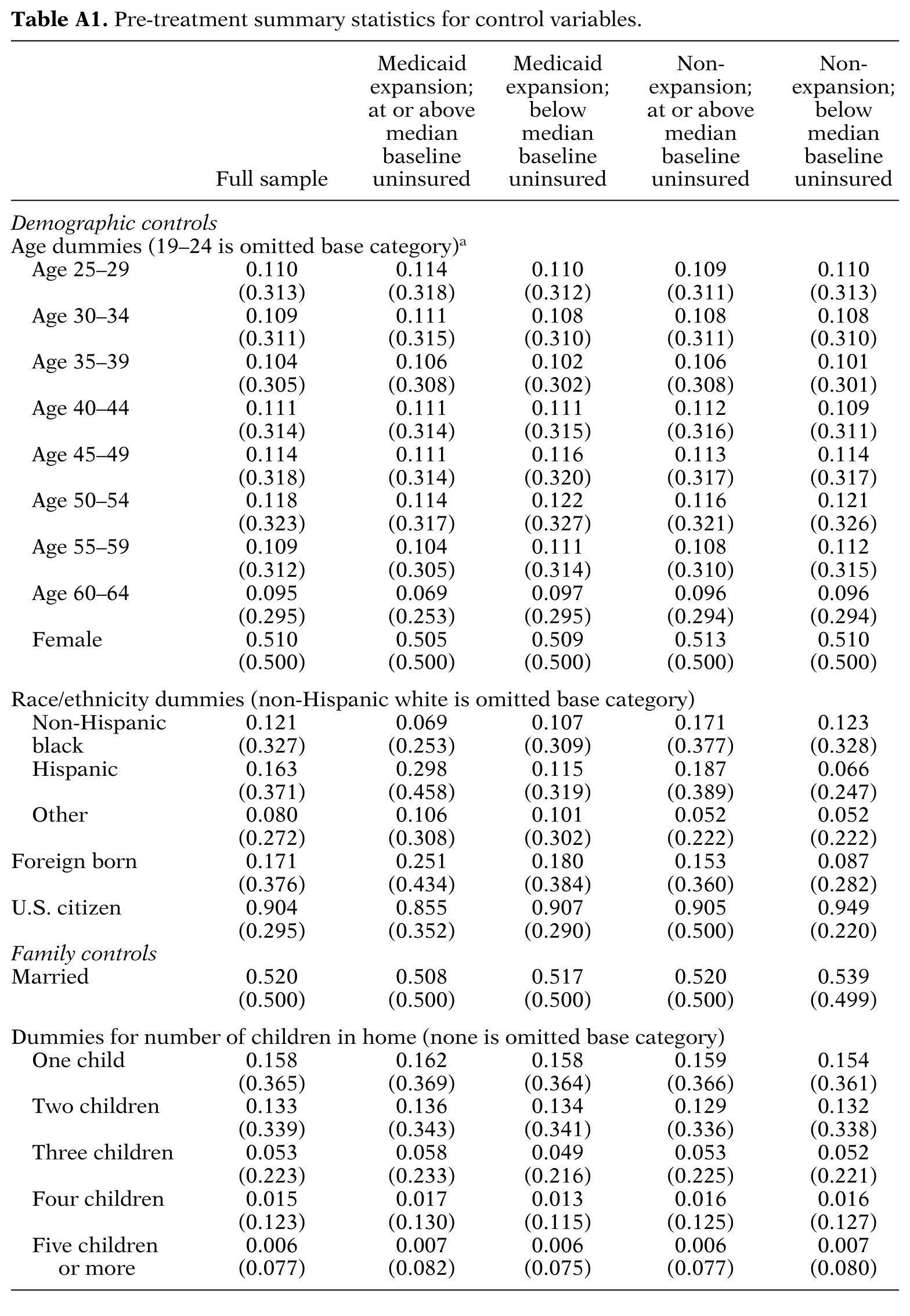
We include a wide range of control variables, divided into several categories. The “demographic” category includes dummies for age (25 to 29, 30 to 34, 35 to 39, 40 to 44, 45 to 49, 50 to 54, 55 to 59, and 60 to 64, with 19 to 24 being the omitted base category), female, race/ethnicity (non-Hispanic black, Hispanic, and other race/ethnicity, with non-Hispanic white being the omitted category), foreign born, and U.S. citizenship status. The next group of controls is “family structure.” This includes dummies for married and the number of children 18 and under in the household (one, two, three, four, and five or more, with zero being the omitted category). 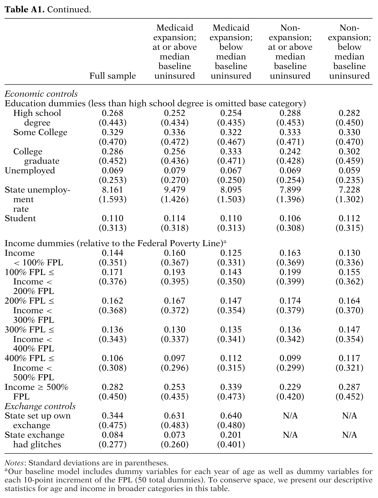The “economic” category features dummies for education (high school degree, some college, and college graduate, with less than a high school degree as the omitted category), household income (separate dummies for each 10-point increment of income as a percentage of the FPL, with the highest category including everyone over 500 percent), whether the respondent reports her primary occupation as student, and whether the respondent is unemployed, as well as one continuous variable: the Bureau of Labor Statistics’ annual state unemployment rate.¹⁵ The final category of controls, which we call “exchange,” includes interactions of the post-treatment dummy with indicators of whether states set up their own private insurance exchanges (as opposed to using the federal exchange) and whether these exchanges experienced glitches. These controls aim to address the possible concern that the decision to expand Medicaid might be correlated with other, harder-to-measure aspects of state involvement with the ACA (e.g., degree of outreach) that could separately influence insurance coverage or health-related outcomes. This information comes from the KFF (2014) and Kowalski (2014).

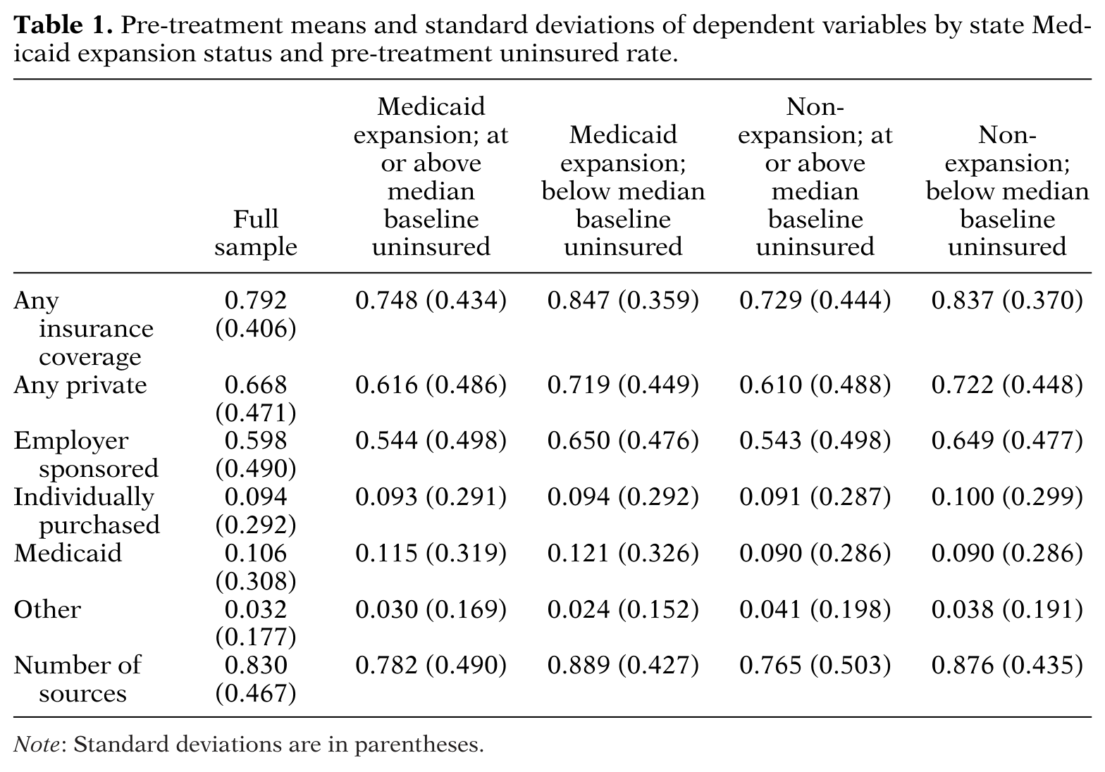
Table 1 provides pre-treatment means and standard deviations of the dependent variables, while Appendix Table A1 does the same for the controls.¹⁶ We also report the summary statistics stratified into four groups based on whether the respondent’s state expanded Medicaid and whether her local area’s pre-treatment uninsured rate was above or below the median for individuals in the sample. Seventy-nine percent of the sample had insurance at baseline, including 11 percent with Medicaid. For both the high- and low-uninsured rate subgroups, individuals in Medicaid expansion states were slightly more likely to have insurance prior to 2014 than those in non-expansion states, with the differences being driven entirely by Medicaid. Our econometric design will account for these baseline differences.

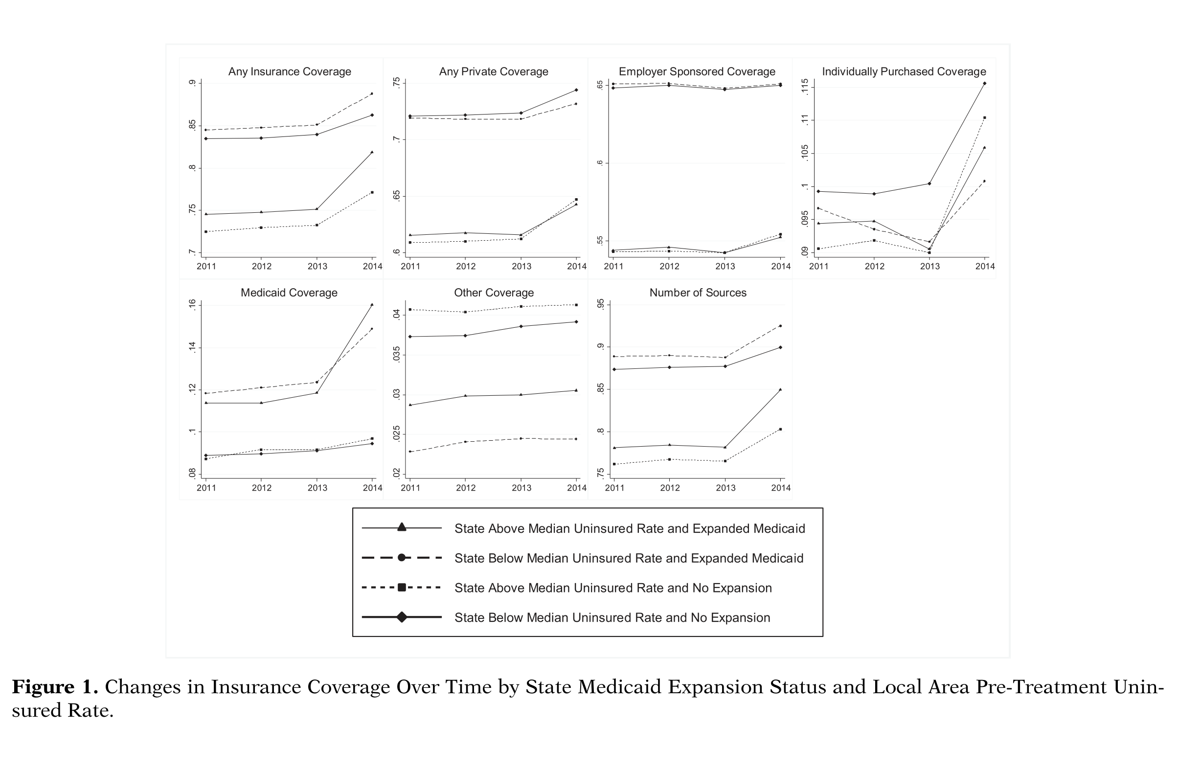
Figure 1 presents changes in our insurance variables of interest during the sample period, stratified into the same four groups. With seven insurance outcomes and four groups per outcome, there are a total of 28 lines. In almost all cases, the pre-ACA trends do not appear to differ meaningfully by state Medicaid expansion status or local area baseline uninsured rate. The only exception is that the “Medicaid expansion—low baseline uninsured rate” group exhibits a trend in privately purchased coverage that is somewhat different from those of the other groups. We therefore view the pre-treatment trends as providing preliminary support for the use of the baseline uninsured rate and Medicaid expansion variables as sources of identification in our econometric models. Increases in the probabilities of having any coverage, privately purchased coverage, any private coverage, and Medicaid are evident in 2014. We next turn to regression analyses to identify the extent to which these increases represent causal effects of the ACA.

Table 1. Pre-treatment means and standard deviations of dependent variables by state Medicaid expansion status and pre-treatment uninsured rate

FULL-SAMPLE ANALYSES

Baseline Models

We begin with a DD specification:

where $y_{iast}$ is the outcome for individual i in local area a in state s in year t, $POS{T}_t$ is an indicator for whether period t is in the post-treatment year of 2014, $MEDICAI{D}_s$ is an indicator for whether state s participated in the ACA’s 2014 Medicaid expansion, $X_{iast}$ is a vector of control variables, ${\alpha }_{as}$ is a local area fixed effect, and ${\epsilon }_{iast}$ is the error term.¹⁷ Standard errors are heteroscedasticity-robust and clustered by state.

represents the effect of the non-Medicaid components of the ACA (insurance market reforms, individual mandate, subsidies, exchanges) while ${\beta }_2$

is the effect of the Medicaid expansion. ${\beta }_1$

• ${\beta }_2$

, therefore, gives the impact of the fully implemented ACA, whereas ${\beta }_1$

is the impact of the ACA without the Medicaid expansion. Interpreting ${\widehat{\beta }}_1$

as causal requires that there would have been no changes in the outcomes in 2014 in the absence of the ACA, conditional on the controls. This is a strong assumption since insurance coverage patterns fluctuate over time. The coefficient estimate ${\widehat{\beta }}_2$

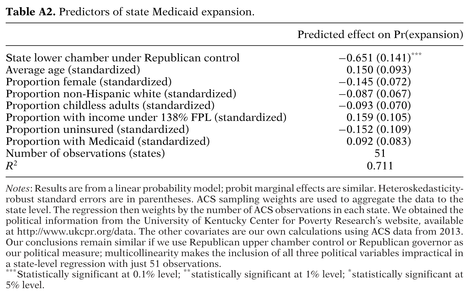
has a causal interpretation under the assumption that, conditional on the other covariates, changes in the outcomes in 2014 would have been the same in expansion and non-expansion states if the expansion had not occurred. This is also a strong assumption given the political nature of the Medicaid expansion decision and the possibility that unobserved determinants of 2014 coverage changes could be correlated with a state’s political climate. Sobel (2014) provides evidence that the Medicaid expansion decision was largely a political calculation, as states with Republican control of the lower chamber, upper chamber, and governorship were all less likely to participate in the ACA’s Medicaid expansion than their counterparts, with lower chamber control being the strongest predictor. In Appendix Table A2, we report results from our own state-level analysis of the determinants of a state’s Medicaid expansion decision. The “Republican lower chamber control” indicator remains the dominant variable in a regression that also includes population demographics (average age, proportion female, and proportion non-Hispanic white), share of the population likely to be eligible for the expansion (proportion of childless adults and proportion below 138 percent of the FPL), and baseline coverage levels (proportion uninsured and proportion with Medicaid).¹⁸

Figure 1. Changes in Insurance Coverage Over Time by State Medicaid Expansion Status and Local Area Pre-Treatment Uninsured Rate

Given concerns about the key identifying assumptions from the DD model, our preferred specification is a DDD specification that exploits variation in the intensity of treatment arising from differential pre-treatment (2013) uninsured rates across local areas. This follows the Finkelstein (2007) and Miller (2012) studies of the effects of the introduction of Medicare and the Massachusetts health care reform, respectively. Adding this layer of geographic variation in the effect of the non-Medicaid portion of the ACA allows us to include time period fixed effects to capture nationwide changes in the outcomes that would have occurred if the ACA had not been implemented, and also to allow for a Medicaid-expansion-state-specific shift in the fixed effect in 2014. Assuming that the extent of an area’s treatment is proportional to its baseline uninsured rate, the DDD model is as follows:

where $UNINSURE{D}_{as}$ is the 2013 uninsured rate in local area a in state s and ${\tau }_t$ is a year fixed effect. Note that $POS{T}_t$ is no longer included in the model since it is perfectly collinear with the year fixed effects, while $MEDICAI{D}_s$, $UNINSURE{D}_s$, and $UNINSURE{D}_s$ × $MEDICAI{D}_s$ are not separately included since they are perfectly collinear with the area fixed effects.

In equation (2), the effect of the ACA without the Medicaid expansion is given by ${\gamma }_1$×$UNINSURE{D}_{as}$, which means it is assumed to be 0 in a (hypothetical) area with a 0 percent uninsured rate at baseline and to increase linearly as the pre-ACA uninsured rate rises.¹⁹ The identifying assumption for the impact of the non-Medicaid expansion components of the ACA is therefore that, in the absence of the ACA, any changes in the outcomes that would have occurred in 2014 would not have varied differentially by local area uninsured rates, conditional on the controls.

Similarly, the effect of the Medicaid expansion is given by ${\gamma }_3$ × $UNINSURE{D}_{as}$. As is the case with the private portion of the ACA, the impact of the Medicaid expansion is now assumed to vary linearly with the baseline uninsured rate. Since it seems reasonable that the Medicaid expansion should not impact insurance coverage in areas with a 0 percent baseline uninsured rate, we consider ${\gamma }_2$ to capture unobserved confounders rather than representing part of the expansion’s causal effect.²⁰ Our identifying assumption for the impact of the Medicaid expansion is therefore that, in the absence of the ACA, the differentials in the insurance outcomes between high and low baseline uninsured rates areas in Medicaid expansion states would have evolved similarly to these differentials in non-Medicaid expansion states. This is a weaker assumption than the corresponding one from the DD specification, which did not allow for any differentials in the evolution of insurance outcomes between Medicaid expansion and non-expansion states aside from those caused by the expansion.

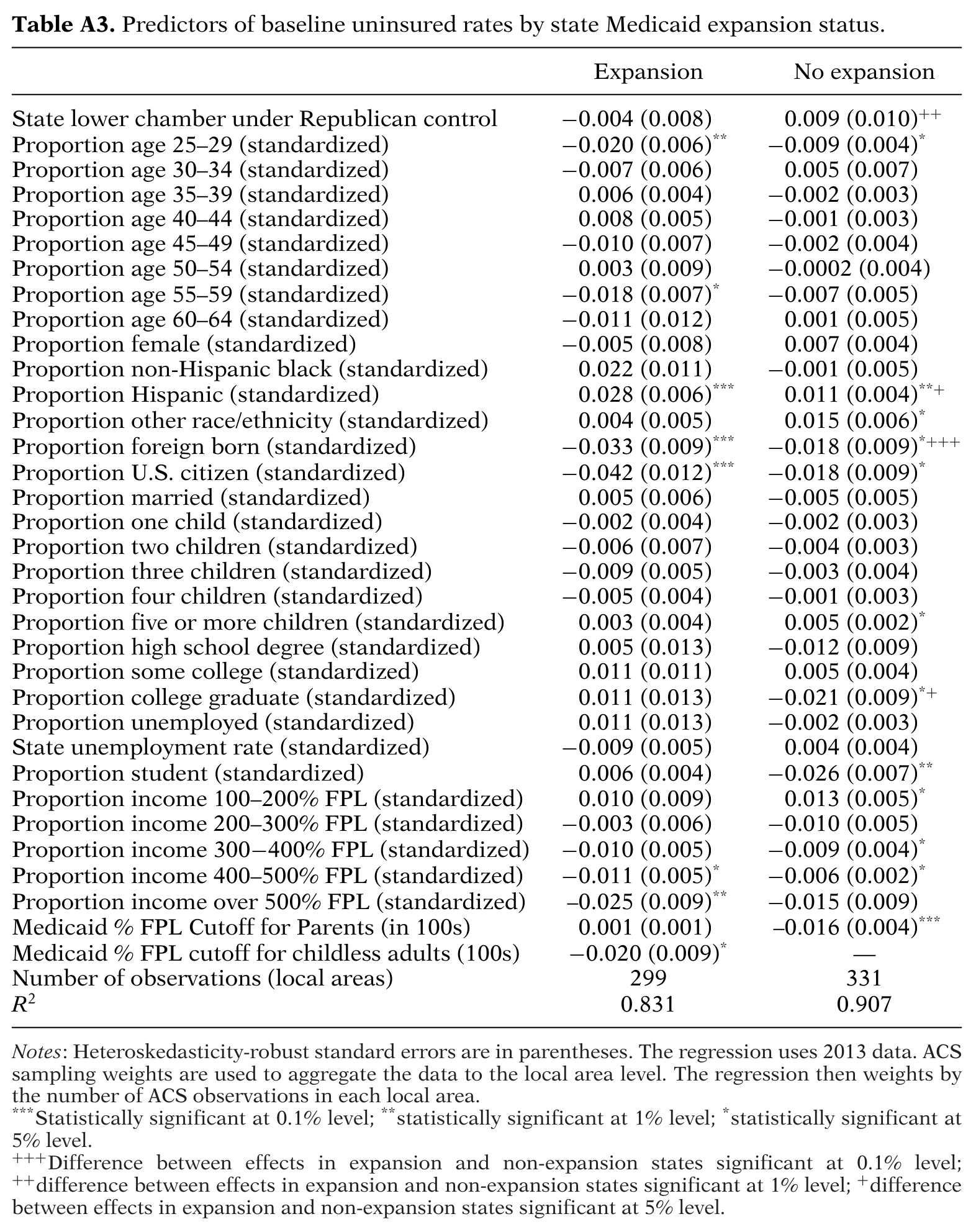
Some preliminary support for the DDD model comes from regressing—separately for Medicaid expansion and non-expansion states—local area baseline uninsured rates on the demographic, family structure, and economic controls along with the pre-ACA Medicaid income eligibility cutoffs for parents and childless adults. As shown in Appendix Table A3, the state-level “Republican lower chamber control” variable is not a statistically significant predictor of 2013 local area uninsured rates in either Medicaid expansion states or non-expansion states.²¹ The DDD model therefore appears less susceptible to concerns about other concurrent policies than the DD model. In addition, only four of the 34 covariates have statistically different (at the 5 percent level) effects on baseline uninsured rates in expansion versus non-expansion states. Since the factors influencing pre-ACA uninsured rates are not generally systematically related to a state’s expansion decision, it seems plausible that counterfactual trajectories in insurance coverage would not substantially differ by Medicaid expansion status either.

Robustness Checks

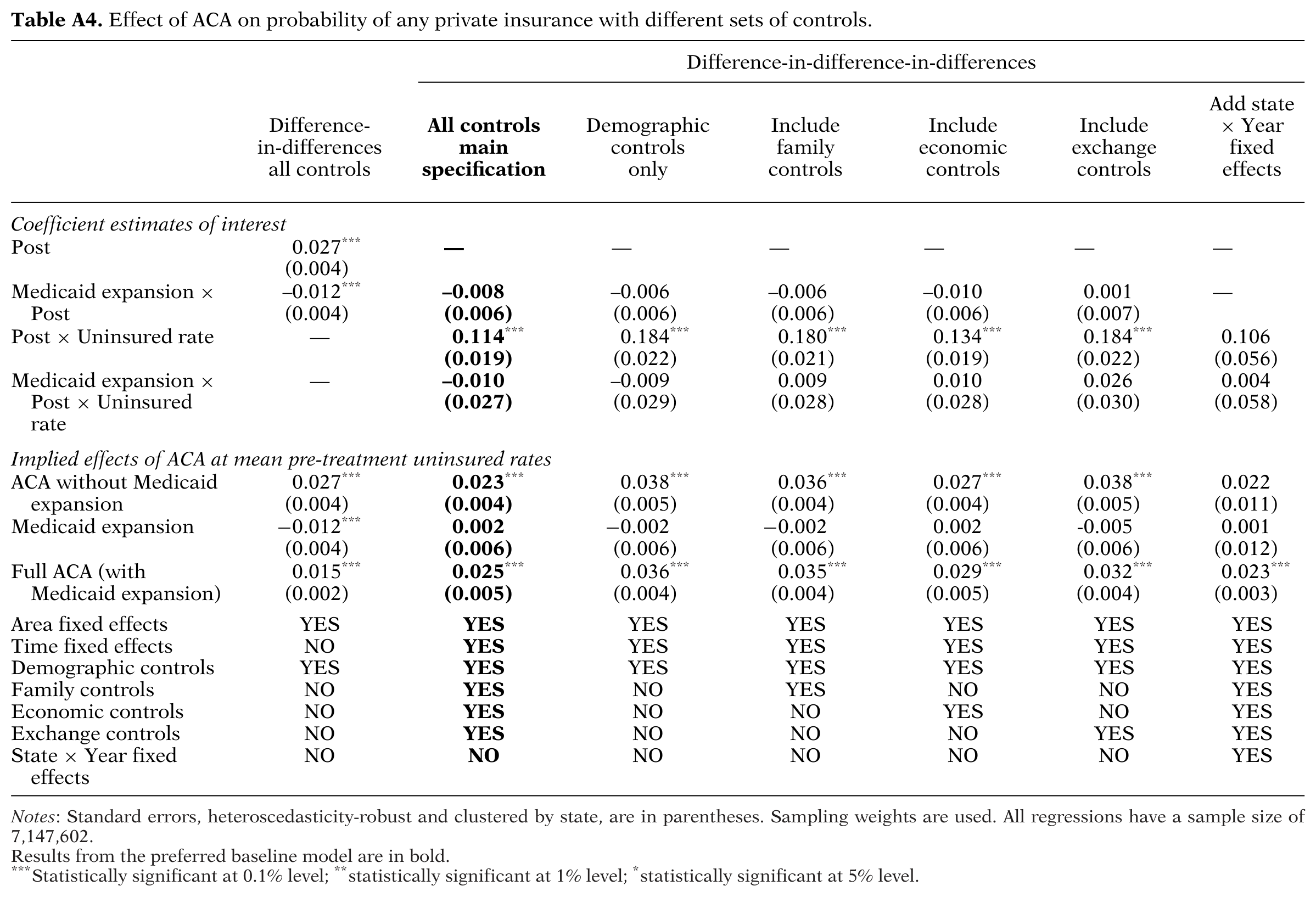
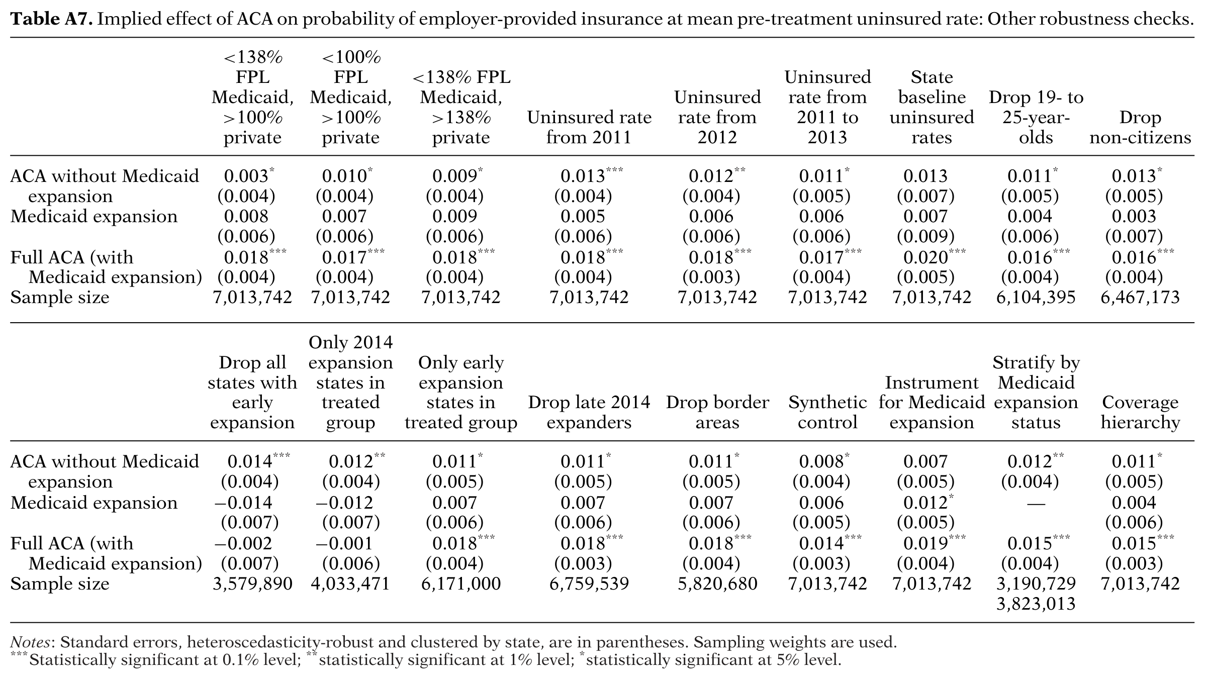
We also estimate a number of variants of the DDD model as robustness checks. The first battery of checks experiments with different sets of control variables. Many of the controls—such as income, unemployment, student status, marital status, and possibly even number of children—could be endogenous to the ACA and therefore lead to an over-controlling problem. We therefore estimate a model that includes only the demographic characteristics age, gender, race/ethnicity, foreign born, and citizenship status. To isolate the influence of each of the other categories of controls, we also estimate models with demographic and family characteristics, demographic and economic characteristics, and demographic characteristics plus the state exchange variables. An additional specification includes all controls as well as a full set of state × year interactions (i.e., separate dummies for each state-by-year combination).

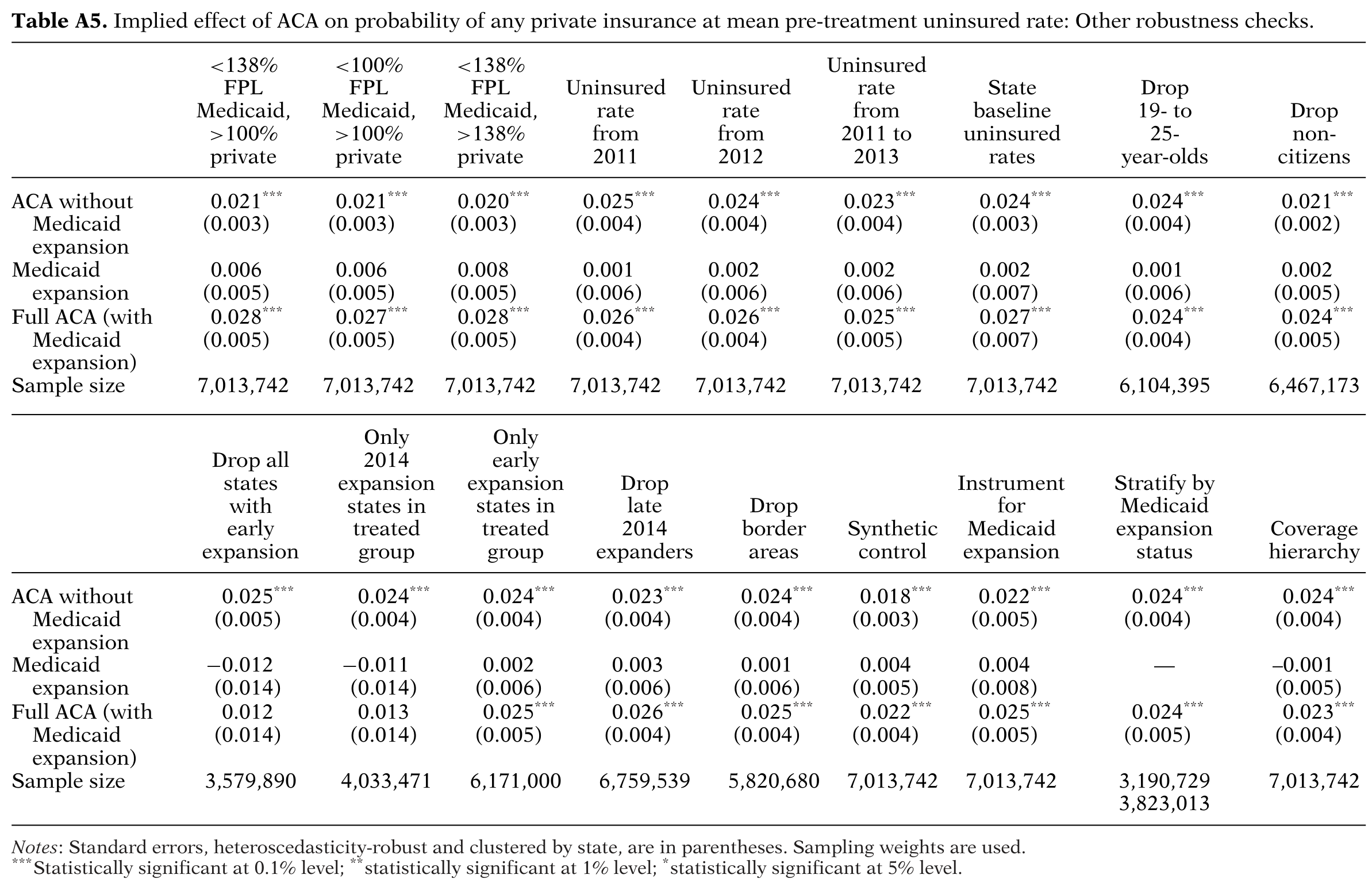
The next group of robustness checks considers different methods of constructing the local area pre-treatment uninsured rates. The first three checks in this category address the issue of whether it is appropriate to interact both $POS{T}_t$ and $MEDICAI{D}_s$ × $POS{T}_t$ with the same uninsured rate variable since the Medicaid expansion and non-Medicaid expansion components of the ACA applied to different populations. Specifically, the Medicaid expansion was for those below 138 percent of the FPL while the exchanges and subsidies were for those above 100 percent of the FPL in states that did not expand Medicaid and above 138 percent in those that did. Consequently, we run a regression that interacts $POS{T}_t$ with the pre-ACA uninsured rate for respondents above 100 percent of the FPL and $MEDICAI{D}_s$ × $POS{T}_t$ with the rate for those below 138 percent of the FPL. We also estimate a similar model using a 100 percent cutoff for both groups and another using a 138 percent cutoff for both groups. The next three robustness checks in this category consider years other than 2013 when constructing pre-treatment uninsured rates. One specification uses only 2011, the second uses only 2012, and the third uses all three pre-treatment years (2011 through 2013). Finally, we estimate a model that defines pre-treatment uninsured rates at the state level rather than the local area level.

The next two robustness checks experiment with dropping groups of individuals with potentially ambiguous treatment statuses. First, we drop 19- to 25-year-olds, the group treated by the 2010 dependent coverage mandate (e.g., Barbaresco, Courtemanche, & Qi, 2015). Recall that the fact that this mandate took effect in 2010 was one of our reasons for starting the sample period in 2011. However, some evidence suggests that the mandate did not reach its full impact until 2012 (Akosa Antwi, Moriya, & Simon, 2013; McMorrow et al., 2015; Sommers et al., 2013), so some individuals in the 19 to 25 age range may have gained insurance from the mandate during our pre-treatment period rather than before it. Second, we drop non-U.S. citizens. Only legal residents are eligible for Medicaid and Marketplace subsidies, meaning that undocumented immigrants should not have been treated. The data do not allow us to distinguish between documented and undocumented immigrants, so we drop all non-citizens and evaluate the robustness of the results.

Next we test the sensitivity of our results to alternative ways of handling early expansion states. Our first robustness check of this type restricts the sample to only the nine treatment states and 20 control states that did not have some form of Medicaid expansion prior to January 2014. This check eliminates any possible confounding from early expansions, but at the cost of discarding potentially useful identifying variation. Second, we estimate separate treatment effects for the treatment states with (18) and without (nine) a prior expansion by running separate regressions for these two groups, in both cases comparing them to the full 24-state control group.

Our next robustness check considers the issue of late, rather than early, expansion. As mentioned, all states’ 2014 Medicaid expansions were effective on January 1, 2014, except Michigan’s, which took effect in April, and New Hampshire’s, which took effect in August. This check therefore drops these two states from the sample.

Concern that individuals living near a border between expansion and non-expansion states might move in order to obtain Medicaid coverage motivates our next robustness check. We drop individuals living in a CBSA that spans multiple states where at least one state expanded Medicaid and one state did not. This results in exclusion of 26 CBSAs.

The next robustness check constructs a “synthetic control group” for the Medicaid-expansion states by building on the approach proposed by Abadie, Diamond, and Hainmueller (2010) for a single treated unit. This technique has been previously applied by other health researchers analyzing state-level expansions (e.g., Kaestner et al., 2015). We first collapse the 27 Medicaid-expansion states into a single treated unit with annual observations and aggregate the non-Medicaid expansion data to the state-by-year level to form a donor pool of states. We then allow the data to select the combination of non-Medicaid expansion states that best matches the expansion states along several dimensions: age, race/ethnicity, foreign born, U.S. citizenship status, marital status, number of children 18 and under in the household, education, household income as percentage of the FPL, and employment/student status from 2011 to 2013 (pooled together) and health insurance status from 2011, 2012, and 2013 (each year included separately).²² The resulting synthetic control group is a weighted average of the 24 states in the donor pool. Following the Fitzpatrick (2008) and Courtemanche and Zapata (2014) applications of this method to individual data, we multiply the ACS weights by the synthetic control weights for non-expansion states, leaving the ACS weights of people living in Medicaid-expansion states unchanged.

Next, we take advantage of the strong influence of politics in determining states’ Medicaid expansion decisions to implement an instrumental variables (IV) strategy. Defining ${\mathrm{R}\mathrm{E}\mathrm{P}}_s$ as an indicator for the state having a Republican-controlled lower chamber in 2013, we use ${\mathrm{R}\mathrm{E}\mathrm{P}}_s$ × $POS{T}_t$ and $UNINSURE{D}_{as}$ × ${\mathrm{R}\mathrm{E}\mathrm{P}}_s$ × $POS{T}_t$ as the two instruments, with $MEDICAI{D}_s$ × $POS{T}_t$ and $UNINSURE{D}_{as}$ × $MEDICAI{D}_s$ × $POS{T}_t$ being the two endogenous variables. The exclusion restriction requires that, conditional on the covariates, the political instruments only influence changes in insurance coverage in 2014 via the endogenous variables.

Another robustness check relates to the fact that, while our identification strategy was inspired by Finkelstein (2007) and Miller’s (2012) use of geographic variation in pre-treatment uninsured rates to identify the effects of Medicare and the Massachusetts reform, the operationalization of this strategy in our context is complicated by the additional layer of variation coming from the Medicaid expansion. We therefore conduct separate regressions for Medicaid expansion and non-expansion states, where for both groups the model is a straightforward difference-in-difference with the only interaction term being $UNINSURE{D}_{as}$ × $POS{T}_t$. This enables an analogous interpretation to Finkelstein (2007) and Miller (2012).

Finally, it has been noted that the ACS produces larger estimates of non-group coverage than other surveys (Mach & O’Hara, 2011). Given our interest in estimating the impact of the ACA on different sources of coverage, our final specification check implements a coverage hierarchy for those with multiple forms of insurance. Following Abraham, Karaca-Mandic, and Boudreaux (2013), we rank coverage as follows: public, then employer-sponsored health insurance (ESI), then direct purchase/non-group plans, then other. After implementing this hierarchy, the percentage of individuals in our sample classified as having non-group/individual coverage falls, as expected (from 9.4 to 6.7 percent).

RESULTS

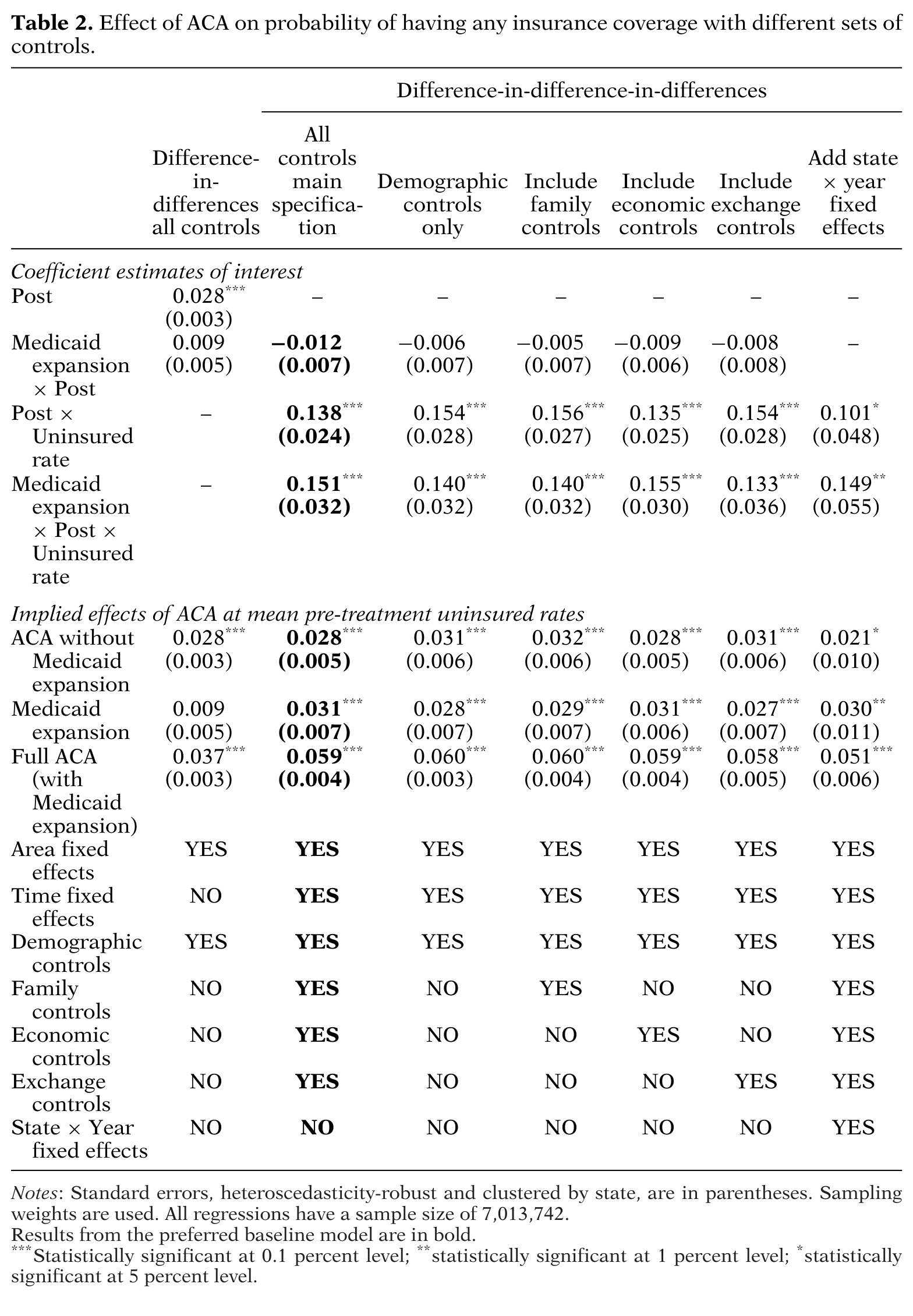
The discussion of our regression results begins with an examination of the estimated effects of the ACA on the probability of respondents having any insurance coverage. Table 2 contains these results for the baseline DD and DDD models and the robustness checks varying the set of controls, while Table 3 reports the results from the other robustness checks. In Table 2, the top panel presents the coefficient estimates for the treatment variables. The bottom panel uses these estimates to compute the implied effects of the private (non-Medicaid expansion) and Medicaid expansion components of the ACA, as well as the full (private plus Medicaid expansion) ACA, at the sample mean pre-treatment uninsured rate. For the DDD specifications, the estimated effects of the private portion, Medicaid portion, and full ACA at the mean are ${\gamma }_1$ × $UNINSURE{D}_{as}$, ${\gamma }_3$ × $UNINSURE{D}_{as}$, and ( ${\gamma }_1$ + ${\gamma }_3$) × $UNINSURE{D}_{as}$, respectively, where $UNINSURE{D}_{as}$ = 0.203 or 20.3 percent.²³

Table 2. Effect of ACA on probability of having any insurance coverage with different sets of controls

Table 3. Other robustness checks

The first column of Table 2 provides the estimates from our “naïve” DD specification. Our coefficient estimate for the post-reform indicator ( ${\beta }_1$) suggests that the 2014 implementation of the non-Medicaid components of the ACA was associated with a 2.8 percentage point increase in the probability of having insurance. The coefficient estimate for the Medicaid expansion/post-reform interaction ( ${\beta }_2$) suggests that expanding Medicaid in 2014 was associated with an additional 0.9 percentage point increase in insurance coverage for the typical expansion state. Taken together, these coefficient estimates ( ${\widehat{\beta }}_1$ + ${\widehat{\beta }}_2$) suggest that full implementation of the ACA was associated with a 3.7 percentage point increase in coverage among non-elderly adults, which is 4.7 percent of the pre-2014 average coverage rate of 79.2 percent.

The second column of Table 2 reports the results from our preferred DDD specification with a complete set of controls. In an area with the average pre-treatment uninsured rate, we estimate that the non-Medicaid components of the ACA increased the coverage rate by 2.8 percentage points while the Medicaid expansion added another 3.1 percentage points. Thus, fully implementing the ACA increased insurance coverage by 5.9 percentage points (or 7.4 percent).

The naïve DD regression therefore appears to substantially understate the effect of the Medicaid expansion, and consequently the effect of the full ACA as well. The DDD model differs from the DD model because of the addition of two terms— $UNINSURE{D}_{as}$ × $POS{T}_t$ and $UNINSURE{D}_{as}$ × $MEDICAI{D}_s$ × $POS{T}_t$ —and also because it attributes any effect of $MEDICAI{D}_s$ × $POS{T}_t$ (the “effect” at zero uninsurance) to endogeneity rather than the causal effect of the Medicaid expansion. Interestingly, the different interpretation of $MEDICAI{D}_s$ × $POS{T}_t$ does not explain the difference in results, as its coefficient estimate is small and insignificant in the DDD regression. Instead, the apparent downward bias in the DD model is due to the omission of $UNINSURE{D}_{as}$ × $POS{T}_t$. In our data, the 2013 uninsured rate was more than 4 percentage points lower in Medicaid expansion states than in non-expansion states, so $UNINSURE{D}_{as}$ × $POS{T}_t$ is negatively related to $MEDICAI{D}_s$ × $POS{T}_t$. Since $UNINSURE{D}_{as}$ × $POS{T}_t$ is positively related to health insurance coverage, its omission leads to downward bias in the coefficient on $MEDICAI{D}_s$ × $POS{T}_t$.

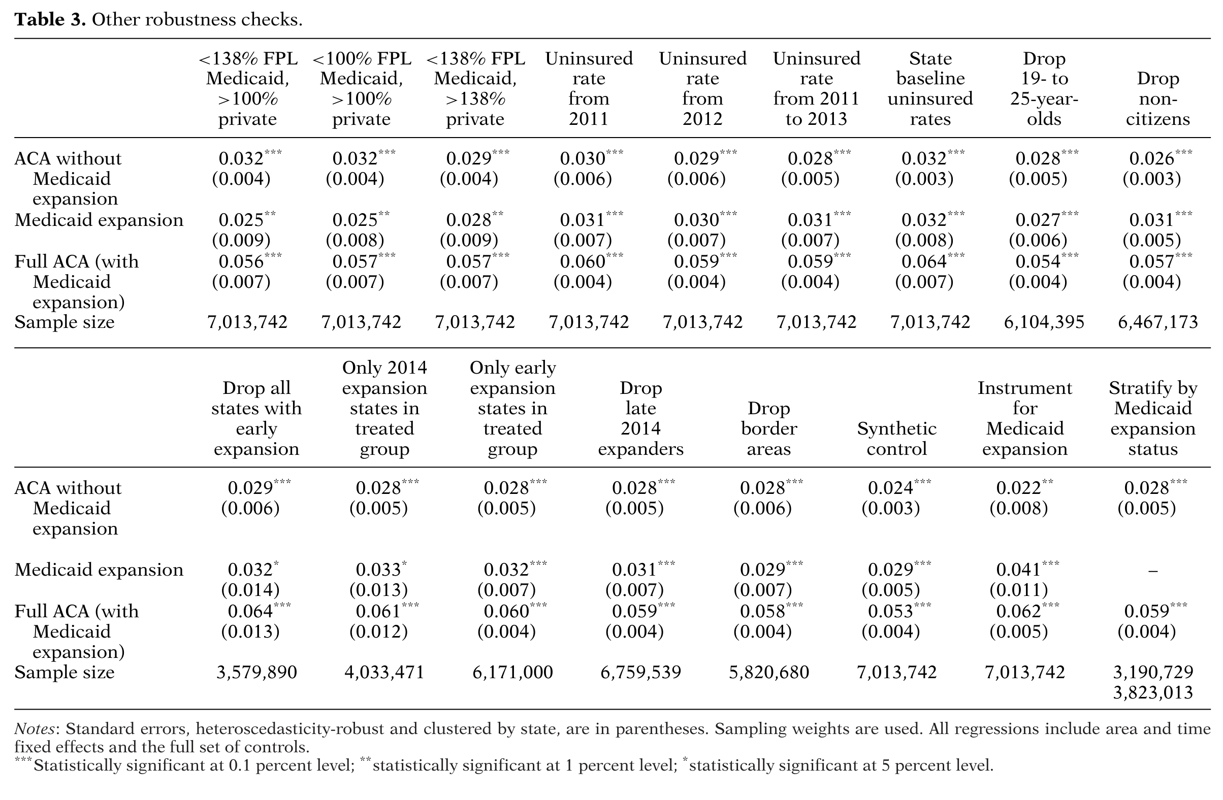
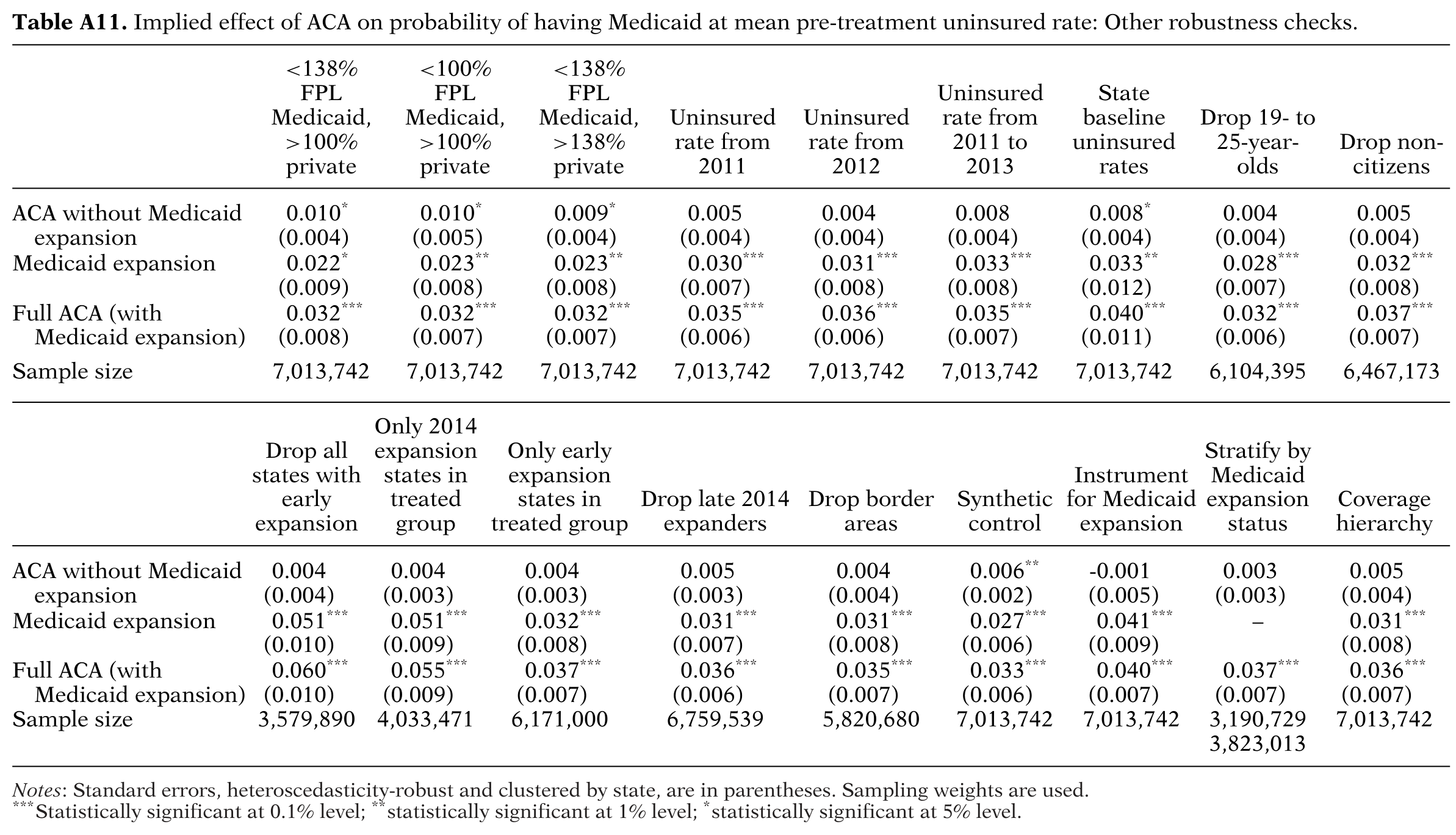
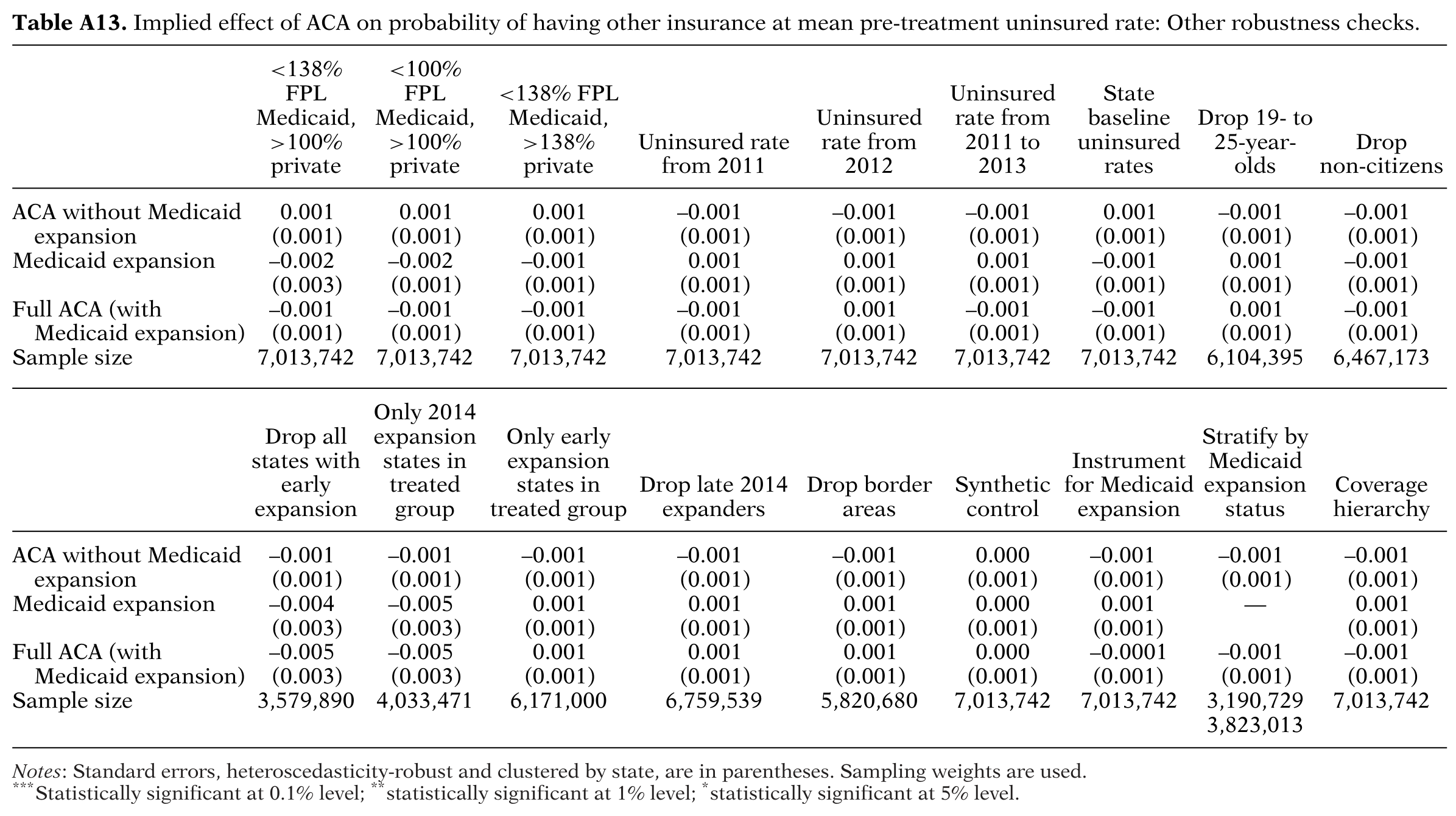
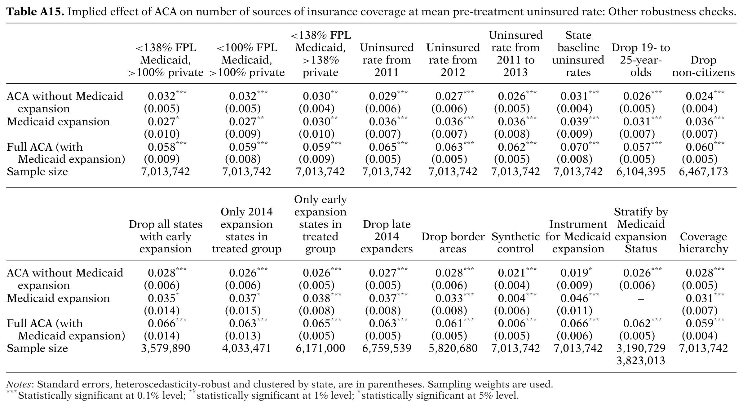
The results from the robustness checks are shown in the next five columns of Table 2 as well as Table 3. Table 2 contains the checks that vary the set of control variables. The first three columns of the top panel of Table 3 show the results from the robustness checks that use percent FPL-based constructions of the pre-treatment uninsured rates, the next three columns use different years to compute the pre-treatment uninsured rates, the seventh column computes these rates at the state rather than local area level, and the last two columns drop individuals for whom treatment is ambiguous due to age or citizenship status. The first three columns of the bottom panel of Table 3 show the results from the checks of the sensitivity of the results to different classifications of early Medicaid expanders. The rest of the bottom panel displays the results from dropping the two late 2014 expansion states (fourth column), dropping border areas (fifth column), implementing the synthetic control design (sixth column), using instrumental variables (seventh column), and running separate DD regressions for Medicaid expansion and non-expansion states (last column).²⁴ The remaining robustness check—the one using the hierarchy of insurance coverage sources—does not apply to the “any coverage” outcome and is therefore excluded from Table 3.

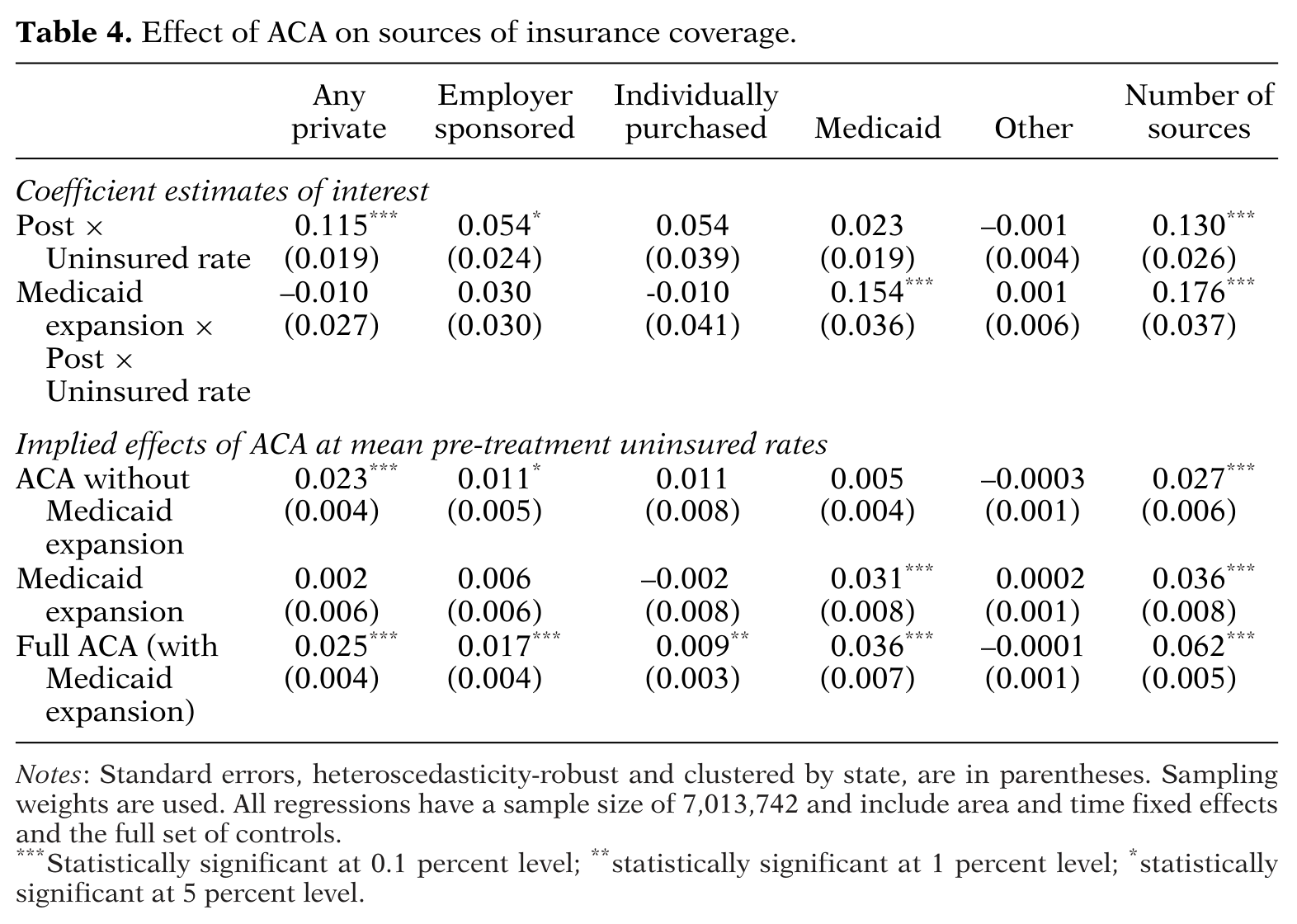
Table 4. Effect of ACA on sources of insurance coverage

Our estimates are remarkably stable across this wide range of specifications and are always statistically significant. At the mean pre-treatment uninsured rate, the estimated effect of the full ACA on the probability of having any coverage varies from 5.1 to 6.4 percentage points across these different specifications. The estimated effects of the non-Medicaid and Medicaid components range from 2.1 to 3.2 percentage points and 2.5 to 4.1 percentage points, respectively.

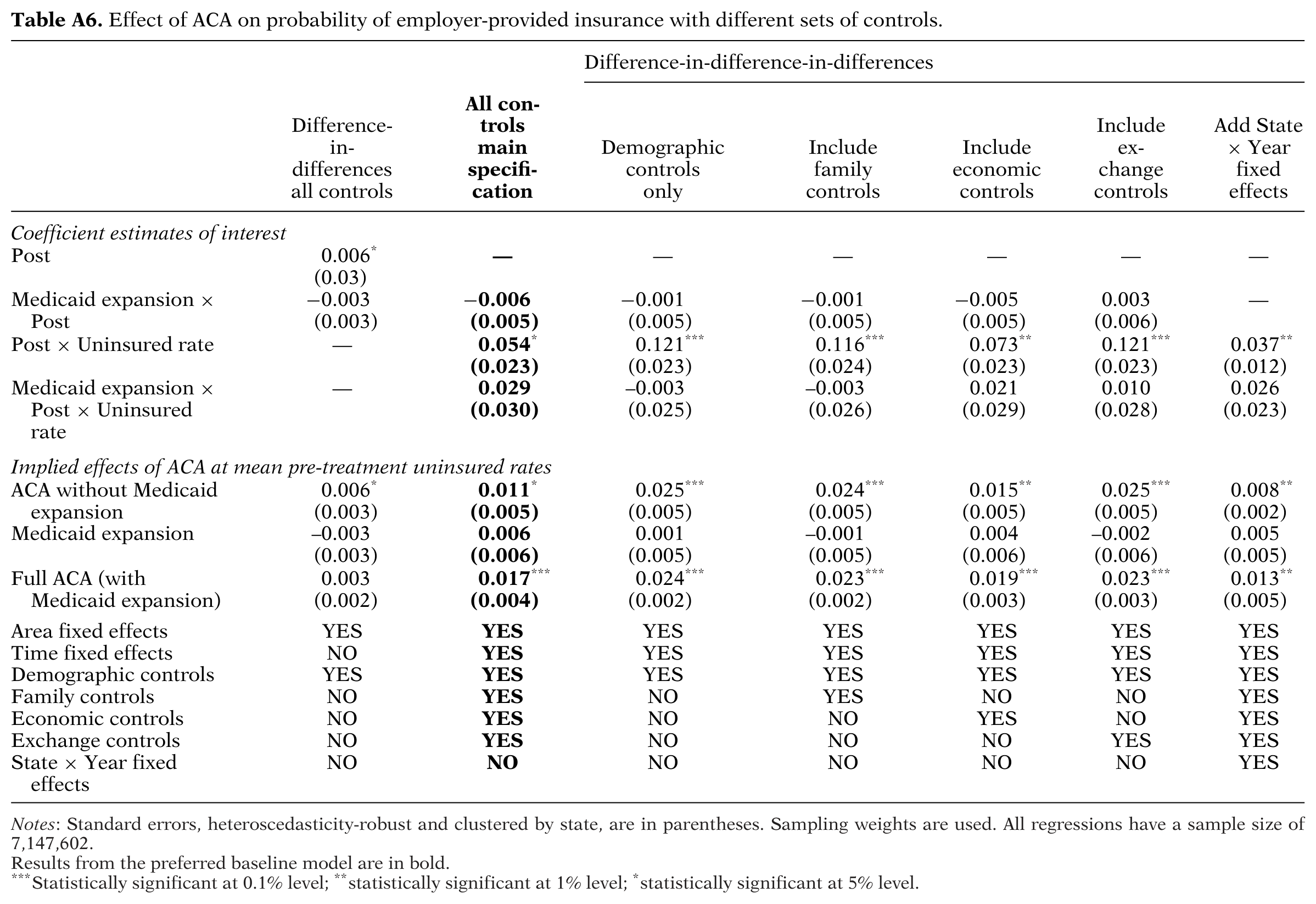
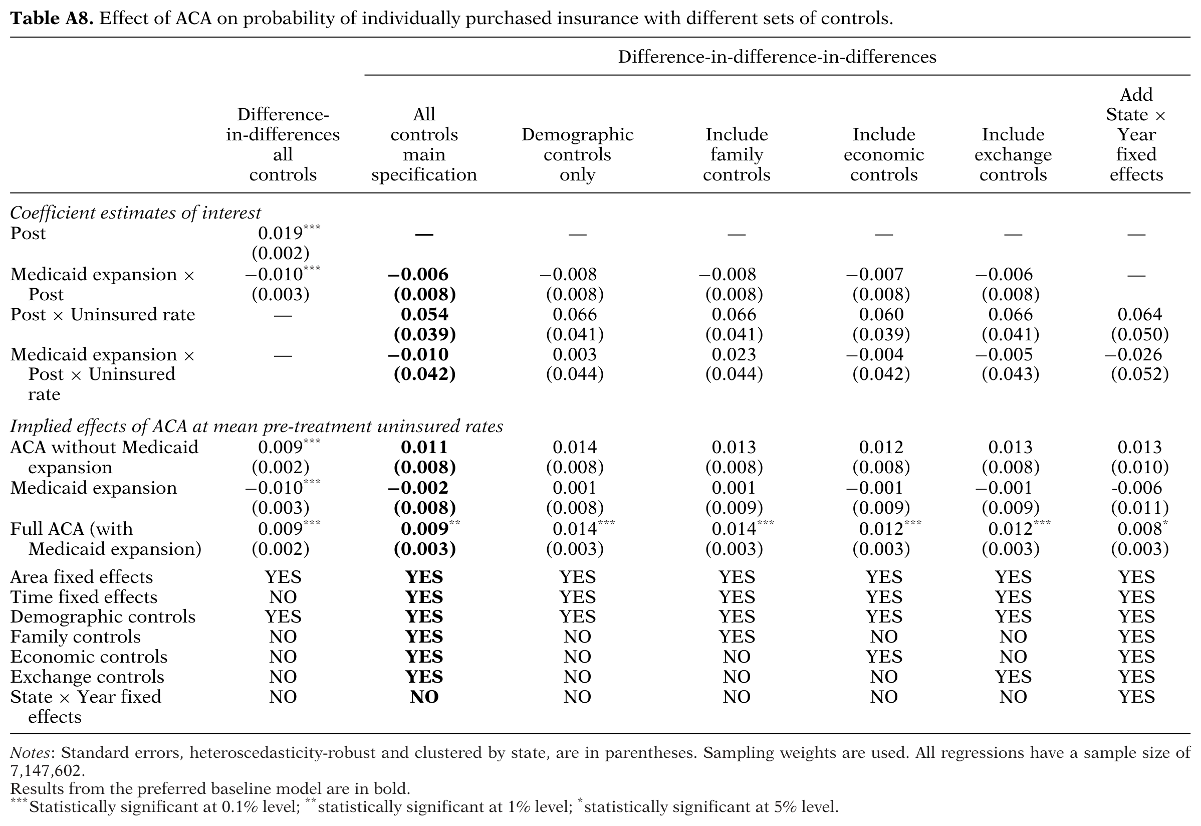
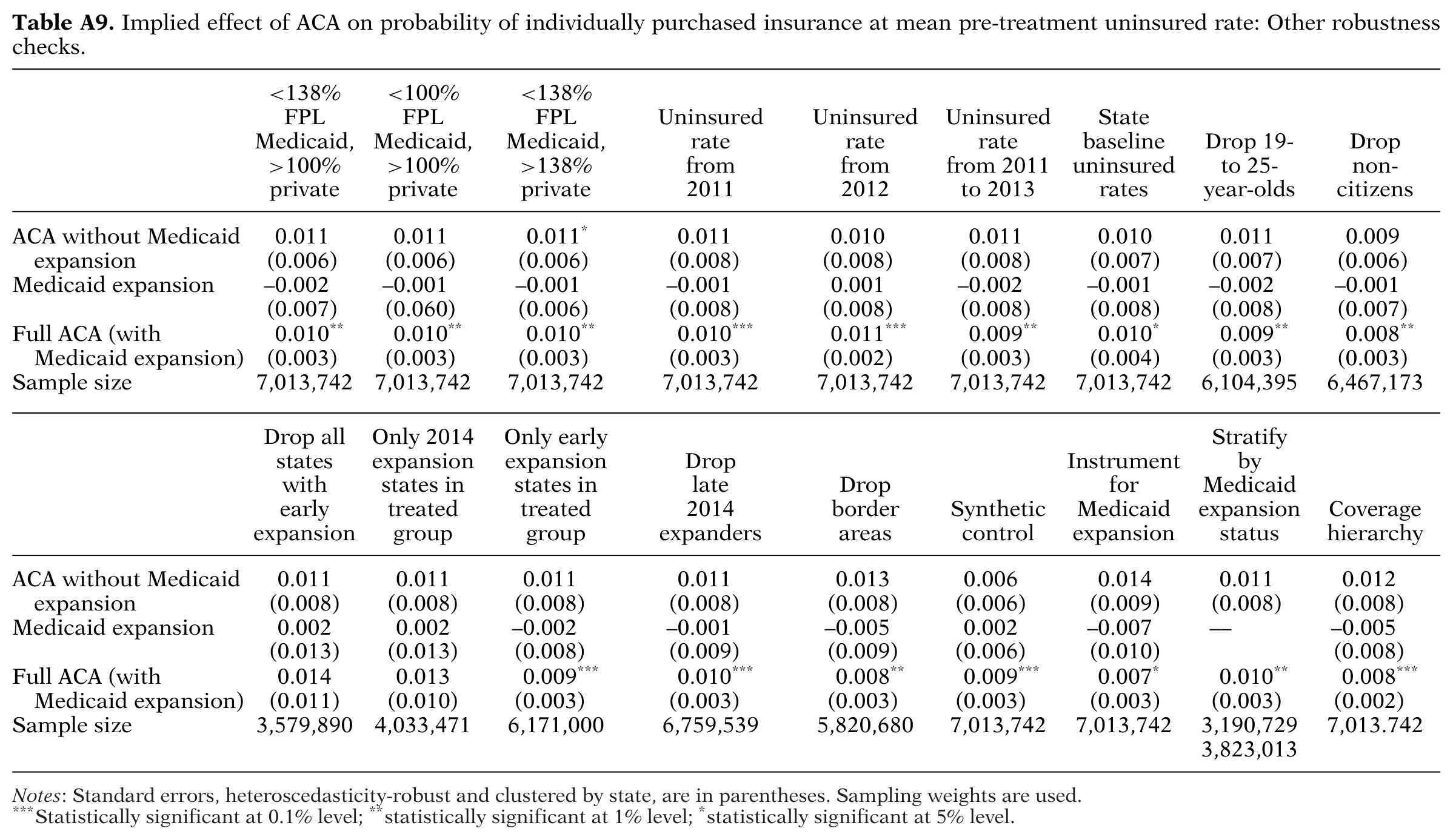
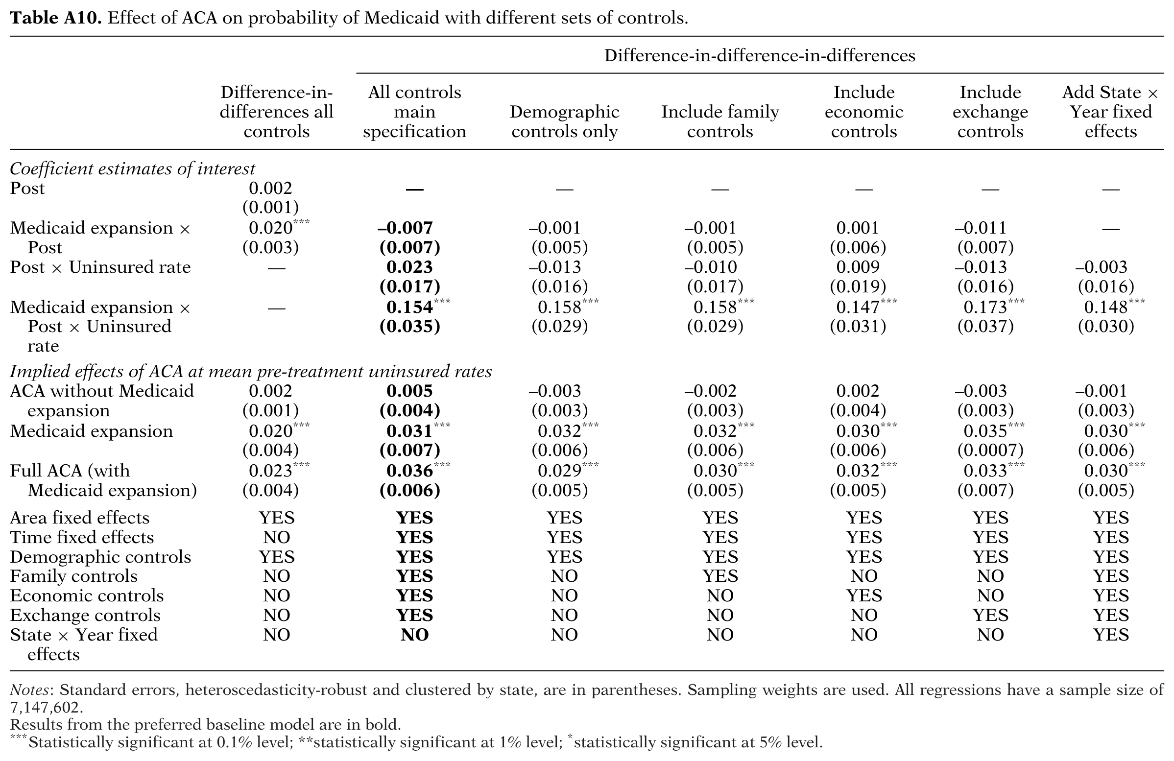
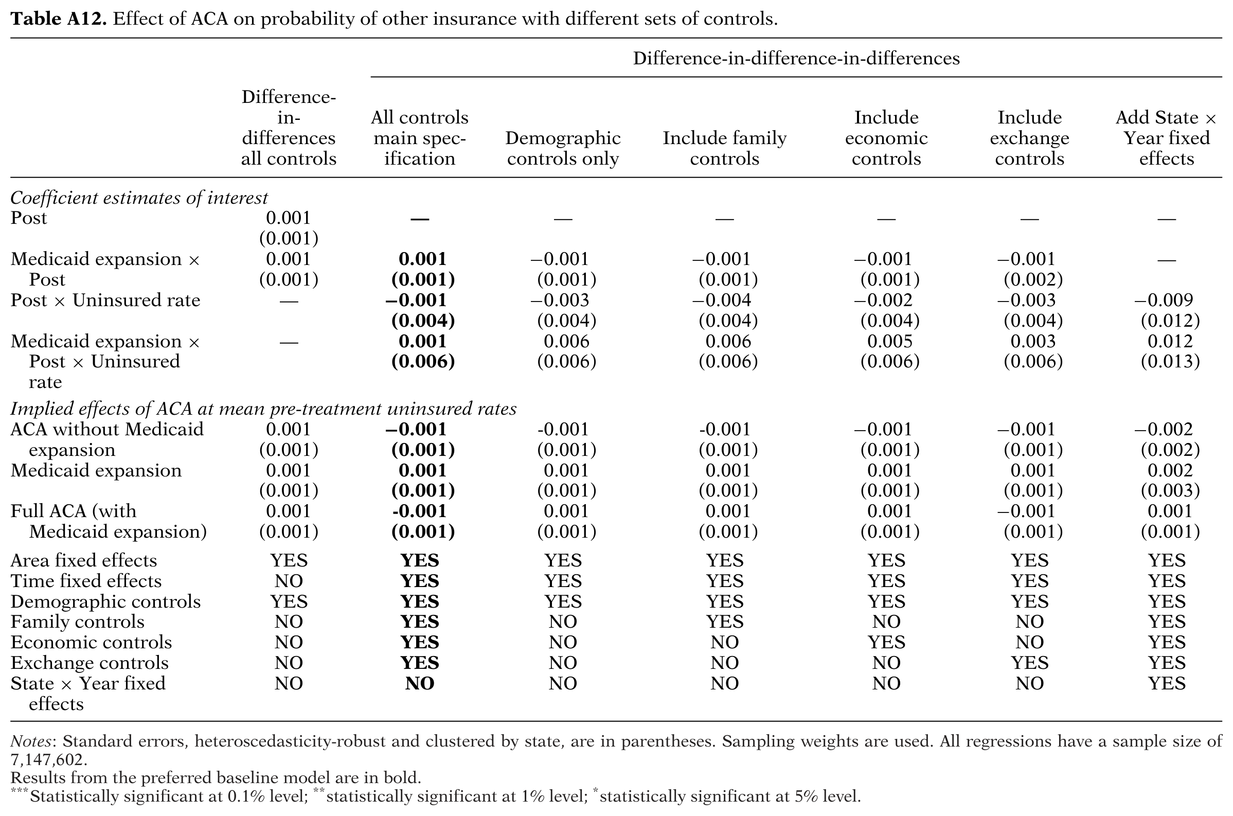
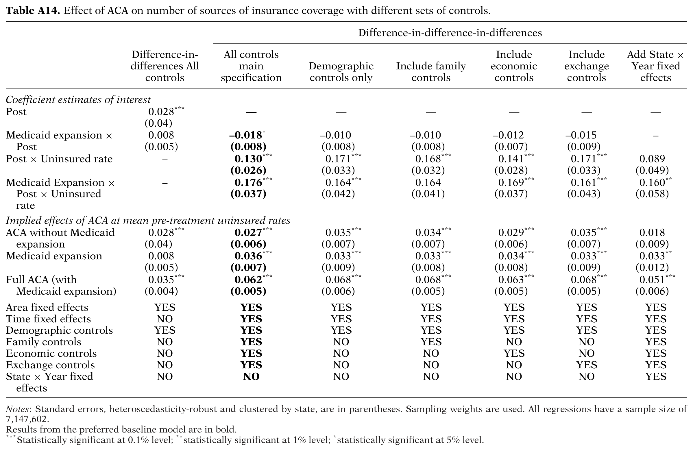
Table 4 shows the estimated effects of the ACA on the sources of coverage using our preferred DDD specification with a complete set of controls. Appendix Tables A4 to A15 present the results from the other specifications for these outcomes.²⁵ The first column of Table 4 shows the results for private health insurance, regardless of whether the coverage is provided by the employer (ESI) or individually purchased. The second and third columns show the effects of the ACA on these two types of coverage separately. The fourth column shows the results for Medicaid coverage, and the fifth shows the effect on any other sources of coverage. Recall that these sources of coverage are not mutually exclusive, so we should not expect, for instance, the sum of the effects on all these sources to be exactly equal to the overall increase in coverage estimated in Tables 2 and 3. This is also the reason why we do not consider econometric models for mutually exclusive choices such as multinomial logits. Finally, the last column of Table 4 uses as the outcome a count variable for the number of sources of coverage.

Our results suggest that the full implementation of the ACA is predicted to increase private coverage by 2.5 percentage points (from the base of 66.8 percent reported in Table 1) in an area with the mean pre-treatment uninsured rate. Surprisingly, this increase in private coverage is mainly due to an increase in ESI rather than additional privately purchased coverage via the exchanges. On average, ESI increased 1.7 percentage points (from a base of 59.8 percent), while individually purchased insurance increased 0.9 percentage points (from a base of 9.4 percent). One possible explanation for the relatively large increase in ESI is the individual mandate, which could increase take-up among employees, their spouses, or their dependents. The employer mandate is not a likely explanation since it had not yet taken effect in 2014, though voluntary early compliance is possible. Another interesting result from the regressions for private sources of coverage is that we find no evidence of crowd-out from the Medicaid expansion. The effects of the Medicaid expansion on having any private coverage, ESI, and individually purchased insurance reported in Table 4 are all very small and not statistically significant.

Results from the fourth column of Table 4 suggest that the ACA Medicaid expansion increased Medicaid enrollment by 3.1 percentage points (29 percent of the base of 10.6 percent) at the mean pre-treatment uninsured rate. In addition, our results show that the fully implemented ACA increased the probability of having Medicaid coverage by 3.6 percentage points, with the remaining 0.5 percentage points coming from the private portion (though this latter estimate is not statistically significant). It seems plausible that the ACA could have induced modest increases in Medicaid take-up—due to the individual mandate or simply heightened awareness of coverage options—even in states that opted out of the Medicaid expansion.²⁶

The fifth column of Table 4 shows that there is no evidence that the ACA affected the probability of having other sources of coverage (e.g., Medicare, Tricare, VA). The estimated effects of the Medicaid expansion and non-Medicaid expansion components, as well as the full ACA, are all very small and insignificant. These null results are not surprising since the ACA deliberately aimed to not disrupt these other types of health insurance coverage.

The last column of Table 4 shows the effects of the ACA on the number of sources of coverage. At the mean pre-treatment uninsured rate, the full ACA increased the number of sources of coverage by 6.2 percentage points, compared to 2.7 without the Medicaid expansion. These estimates are both highly statistically significant and very similar in magnitude to the effects on the probabilities of having any coverage from Tables 2 and 3. This similarity reflects the fact that most insured individuals (96.18 percent in 2013 and 96.24 percent in 2014 in our sample) have only one source of coverage.²⁷

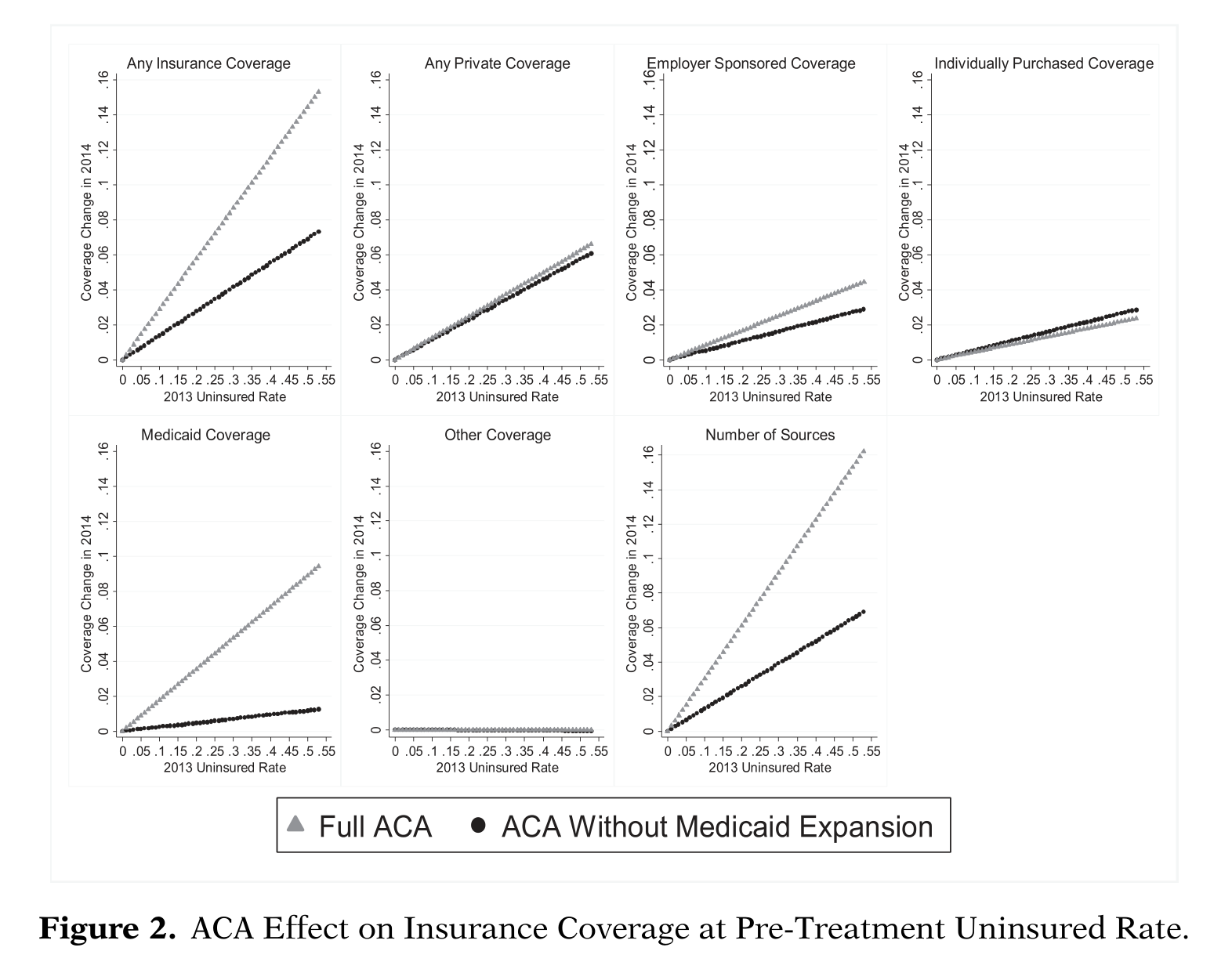
Tables 2 to 4 only compute impacts of the ACA at the mean pre-treatment uninsured rate of 20.3 percent. This approach masks considerable heterogeneity in the law’s effects since local area pre-treatment uninsured rates varied widely, ranging from 3 to 53 percent with a standard deviation of 7 percent. Figure 2 therefore shows how the predicted changes in coverage vary across this range of uninsured rates in both expansion and non-expansion states. We see that for practically every type of coverage the larger the proportion of population uninsured in 2013 in the state, the larger the gain in coverage. The only exception is the “other source of coverage” category for the ACA without a Medicaid expansion, and this is highly statistically insignificant.

Figure 2. ACA Effect on Insurance Coverage at Pre-Treatment Uninsured Rate

More specifically, the top left graph on Figure 2 shows that the predicted impact of the full ACA on the probability of having any coverage reached as high as 15.3 percentage points at the highest sample pre-treatment uninsured rate (53 percent). In contrast, without the Medicaid expansion the maximum effect was only 7.3 percentage points. We find similar maximum effects on the “number of sources coverage” with and without the Medicaid expansion (16.2 and 6.9 percentage points) presented in the bottom right corner of Figure 2. Not surprisingly, these differences in maximum impacts are due entirely to differences in the increases in Medicaid coverage. The “Medicaid coverage” graph predicts increases in Medicaid coverage that reach as high as 9.4 and 1.2 percentage points in expansion and non-expansion states, respectively.

In the cases of any private, employer-provided, individually purchased, and other coverage, the coverage effects may appear slightly different in Medicaid expansion versus non-expansion states, but these differences are never statistically significant at any level of un-insurance. We therefore focus on the results for the full ACA, including the Medicaid expansion. At the highest uninsured rate of 53 percent, we estimate that the full ACA increased private coverage by 6.6 percentage points, increased ESI by 4.5 percentage points, increased individual coverage by 2.4 percentage points, and had no significant effect on other coverage.

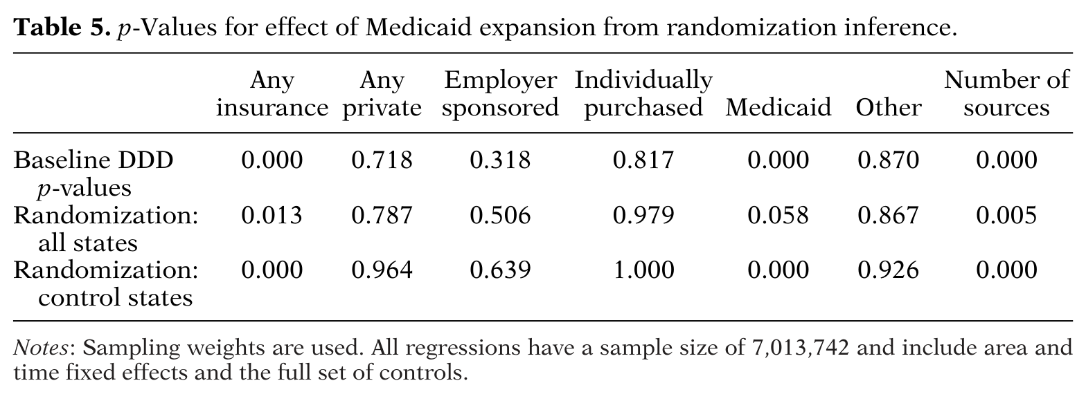
Table 5. p -Values for effect of Medicaid expansion from randomization inference

TESTS RELATED TO INFERENCE

This section conducts inference based on randomization to help rule out the possibility that the statistical significance observed in the baseline regressions is due to underestimated standard errors. This technique has been used to conduct inference in situations where there are few treated (or control) units, which can lead to biased clustered standard errors (e.g., Kaestner, 2016; Kaestner et al., 2015). Since we cluster at the state level, we have 51 clusters with a roughly even split of “treatment” and “control” units with regard to the Medicaid expansion. This is a sufficiently large number of clusters that we would not expect major underestimation of the standard errors, but some underestimation is nonetheless possible (Bertrand & Mullainathan, 2004; Cameron & Miller, 2015).

Following Kaestner (2016); Small, Ten Have, and Rosenbaum (2008); and Rosenbaum (2002) we implement this method by randomly assigning Medicaid expansion status to 27 (the number of states that expanded Medicaid) out of the 51 states in our sample and then re-estimate our DDD model. We repeat this procedure 1,000 times and obtain the null distribution of the DDD estimate. If our baseline DDD estimate is extreme (i.e., lies in the tails of the distribution), then we should reject the null hypothesis. We calculate the p -values of the two-sided tests as the proportion of estimates from the null distribution that are larger (in absolute value) than our DDD baseline coefficient estimate. As an alternative strategy, we repeat the above but use only the 24 non-expansion states, assigning 12 a placebo Medicaid expansion status in each iteration.

Table 5 shows the p -values for the coefficient estimate on the triple-interaction term $UNINSURE{D}_{as}$ × $MEDICAI{D}_s$ × $POS{T}_t$ using randomization inference. The first row shows the p -values calculated based on the clustered standard errors shown previously. The second row shows the p -values based on randomization inference using all 51 states, while the third row uses just the 24 “control” states. While there is some modest sensitivity in the p -values to the use of randomization inference, we do not view this as being large enough to affect our conclusions. The most consequential difference is that the p -value for the effect of the Medicaid expansion on Medicaid coverage rises to slightly over 0.05 using randomization inference with all 51 states. However, this $p$-value shrinks back to <0.00 with just the 24 non-expansion states.

TESTING FOR DIFFERENTIAL PRE-TREATMENT TRENDS

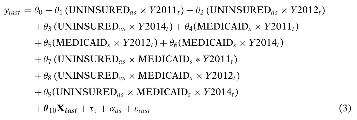
As discussed, identification of the parameters of interest in our models relies on two key assumptions. Conditional on the controls, if the ACA had not occurred (i) changes in insurance coverage in 2014 would not have been correlated with pre-treatment uninsured rates, and (ii) any differential changes in coverage in 2014 between Medicaid expansion and non-expansion states would not have been correlated with pre-treatment uninsured rates. It is not possible to directly test these assumptions since we cannot observe the counterfactual. However, we can indirectly assess the likelihood of these assumptions holding by estimating an event study model that interacts the treatment variables with the full set of year fixed effects, leaving 2013 as the base year. The regression takes the form:

where $Y{2011}_t$, $Y{2012}_t$, and $Y{2014}_t$ are indicators for whether year $t$ is 2011, 2012, and 2014, respectively. The tests for differential pre-treatment trends (i.e., falsification tests) are provided by evaluating whether the coefficients on the “treatment” variables in the pre-treatment years (${\theta }_1$, ${\theta }_2$, ${\theta }_7$, ${\theta }_8$) are equal to 0.

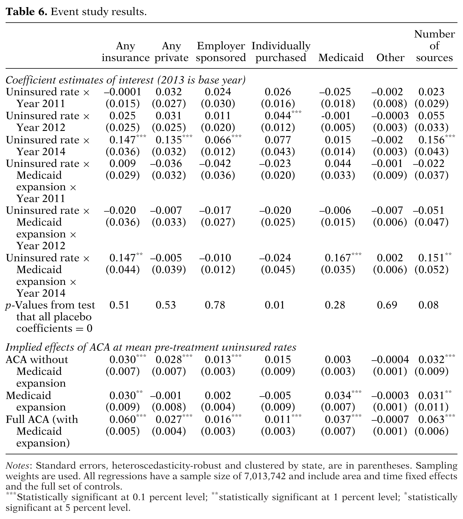
Table 6 presents the event study results for each of the seven outcomes using the full set of controls. The top panel presents the coefficient estimates of interest. There are a total of 28 falsification tests (four parameters of interest in each of seven regressions) and only one significant result at the 5 percent level. One out of 28 is 3.6 percent, so we reject the null hypothesis slightly less often than would be expected by chance. For each regression, the table also reports the p -value from an F -test of the joint significance of the four placebo coefficients. The F -test only rejects the null hypothesis of joint insignificance in the one regression (out of seven) with an individually significant placebo coefficient. These results therefore provide reassurance about the validity of our model to estimate causal effects for the “true” ACA.

The bottom panel of Table 6 uses the results from the 2014 interaction terms to compute the effects of the ACA without the Medicaid expansion, the Medicaid expansion, and the full ACA. The estimated impacts of the “true” ACA, shown in the bottom panel, are very similar to those from Tables 2 and 3.

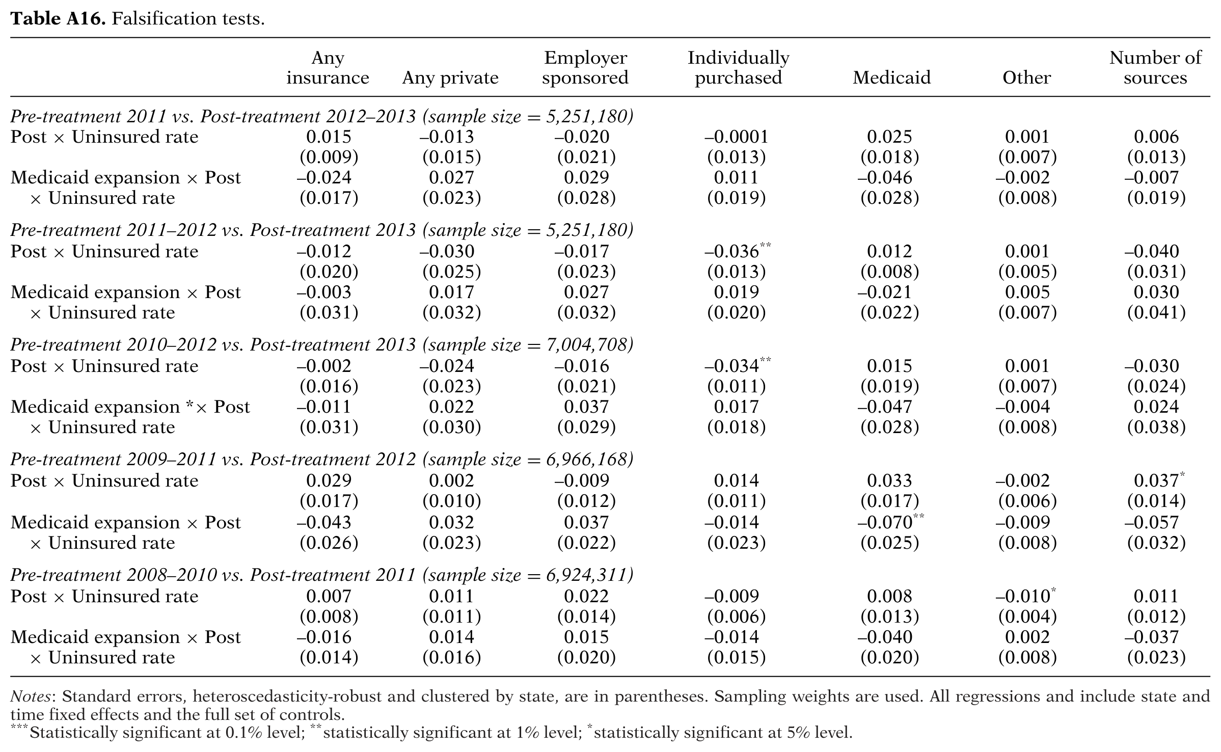
Another way to evaluate the assumption of common pre-treatment trends is to restrict the sample to the pre-treatment period and test whether “placebo” interventions during the pre-treatment years are associated with significant changes in coverage using the same DDD model as our main specification, following Slusky (2016). We present results from several such tests in Appendix Table A16.²⁸ The first two sets of regressions use only the pre-treatment waves from our main sample—2011 to 2013—and define the placebo treatment to occur either at the end of 2011 or the end of 2012. The remaining tests incorporate older waves of the ACS to enable the use of the same four-year time span as our main regressions. Specifically, we use 2010 to 2013, 2009 to 2012, and 2008 to 2011, with the placebo “treatment” occurring in the last year.

Table 6. Event study results

As with the event study analysis, we see roughly the same amount of null hypothesis rejections as would be expected due to chance: five out of 70 (7.1 percent) at a 5 percent significance level.

SUBSAMPLE ANALYSES

Our baseline DDD model described in equation (2) does not allow our estimates of the impact of the ACA to vary by any of the demographic characteristics contained in $X_{iast}$, such as education, race/ethnicity, age, gender, or marital status. Because we expect the impact of the ACA to differ in a meaningful way across demographic groups, we estimate a series of subsample regressions in order to assess the magnitude of these differences. In general, we expect that demographic groups with the highest pre-treatment uninsured rates generate the largest gains in coverage in 2014. Thus, everything else being equal, we would expect larger gains in coverage for non-whites, individuals with relatively low education levels, young adults, men, and unmarried individuals.

Table 7. Education subsamples

In addition, the design of the subsidies for exchange coverage, the fact that several states opted out of the Medicaid expansion, and the nature of pre-ACA Medicaid eligibility requirements combine to generate the potential for further differential gains across demographics such as socioeconomic status, age, and the presence of children in the home.

For each subsample, we re-compute the pre-treatment uninsured rate using only individuals within that particular subsample. Since each subsample must therefore contain enough respondents in 2013 to precisely compute uninsured rates at the local level, we are constrained to a maximum of two or three subsamples for each of our demographic stratifications. For instance, we might ideally prefer to stratify our sample into four race/ethnicity subsamples—non-Hispanic white, non-Hispanic black, Hispanic, and other—but some of our local areas have such a low proportion of blacks or Hispanics that the ACS sample size from those areas is insufficient to credibly compute pre-treatment uninsured rates. Consequently, we only separate the sample into non-Hispanic whites versus others.

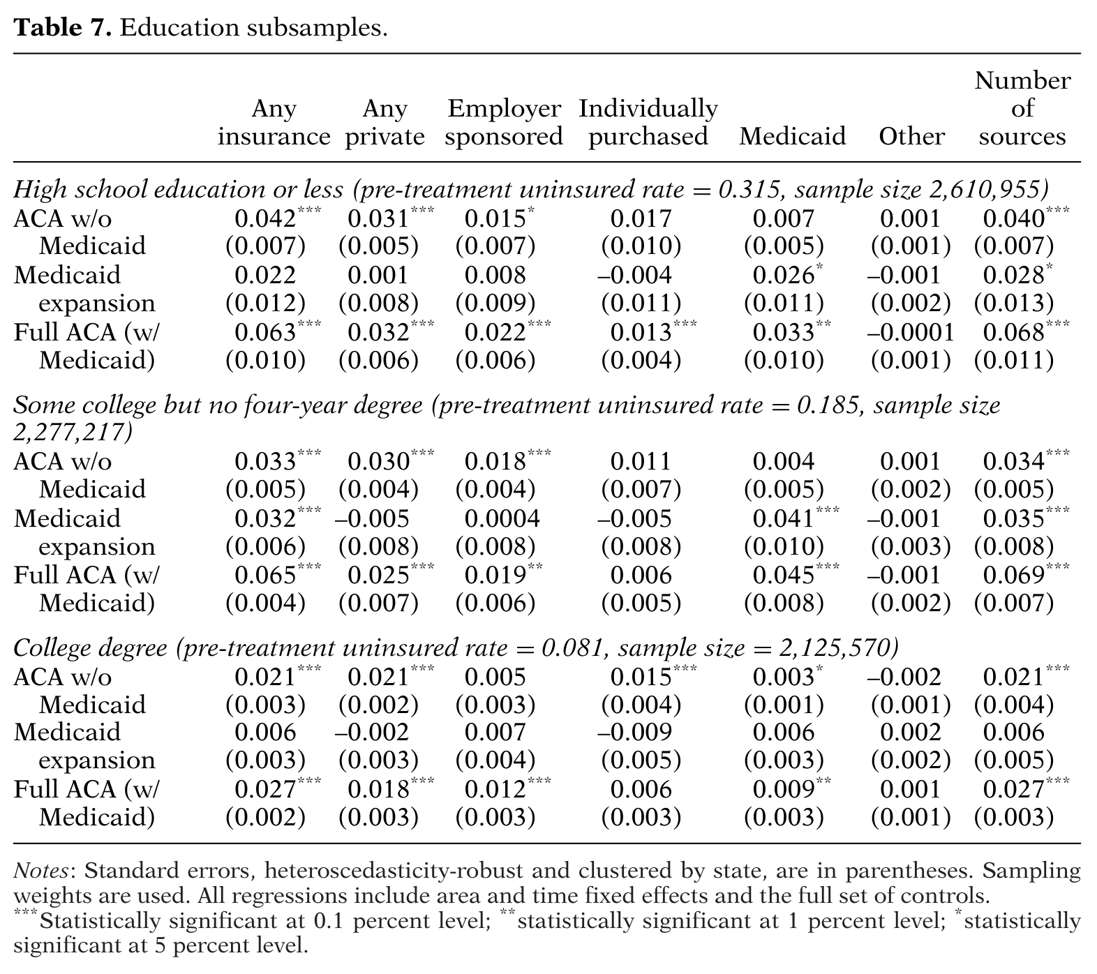
Table 7 presents the results of a stratification of our sample into three groups based on education: those with a high school education or less, those with some college but no four-year degree, and college graduates. Following Kaestner et al. (2015), we use education level rather than income for our evaluation of heterogeneity by socioeconomic status since income could potentially be endogenous to health care reform. Nonetheless, we have verified that if we stratify by income we observe the same general pattern of results.

Our results suggest that, in expansion states, the largest effects on insurance coverage occurred among the two lowest education subsamples. Full implementation of the ACA is predicted to increase coverage by 6.3 percentage points (from a base of 68.5 percent) for those with a high school education or less and 6.5 percentage points (from a base of 81.5 percent) for those with some college but no degree. For both groups, sizeable shares of the gains come from both private insurance and Medicaid: 3.2 and 3.3 percentage points, respectively, for the high school group and 2.5 and 4.5 percentage points, respectively, for the “some college” group. It is noteworthy that the “some college” group experienced a larger gain from the Medicaid expansion. This could perhaps be attributable to the high school group being more likely to be eligible for Medicaid prior to the ACA expansion. Another interesting result for the two lower-education subsamples is that we find no evidence that the Medicaid expansion crowded-out private coverage: the effects of the Medicaid expansion on the probability of having private insurance are small and insignificant for both subgroups.

Turning to the results for the subsample of individuals with college degrees, full implementation of the ACA is predicted to increase coverage by a more modest 2.7 percentage points (from a base of 91.9 percent). An increase in private coverage appears to be the main driver of these gains, as full ACA implementation increased private coverage by 1.8 percentage points, accompanied by a smaller increase in Medicaid coverage (0.9 percentage points). Two-thirds of the gains in private coverage come from an increase in employer-provided coverage.

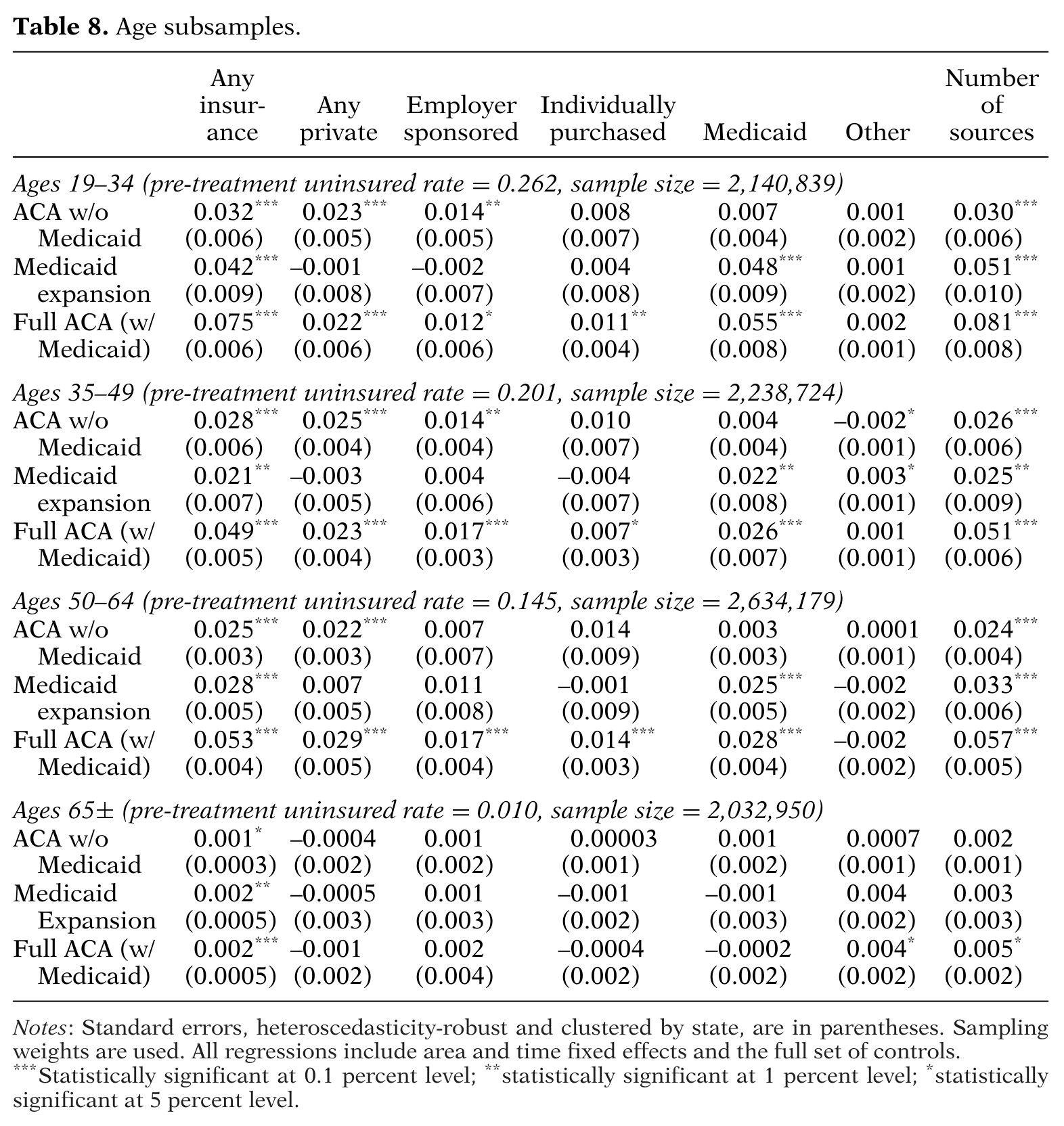
Next we stratify the sample by age. We divide our main sample into three categories: those 19 to 34, those 35 to 49, and those 50 to 64. We also include an additional subsample—those 65 and older—since this group should not have been affected by the ACA and therefore provides the opportunity for a falsification test. Table 8 reports pre-treatment uninsured rates that decline with age prior to Medicare eligibility, falling from 26.2 percent for those 19 to 34 to 14.5 percent for those 50 to 64. The reason for being uninsured likely differs by age, with the relatively young possibly viewing health insurance as an unnecessary expense given their good overall health, while older individuals may have trouble finding affordable coverage due to poor health. Given the individual mandate, both groups may find exchange coverage attractive for different reasons, such as the potential for a premium subsidy (benefiting the young) and the presence of a more diverse risk pool (benefiting the old). Table 8 shows that the largest gain in coverage is for the 19- to 34-year-old group. Full implementation of the ACA is predicted to increase coverage by 7.5 percentage points among this group compared to 4.9 percentage points among 35- to 49-year-olds and 5.3 percentage points among 50- to 64-year-olds. For all three non-elderly groups, increases in Medicaid coverage account for more than half of the increase in coverage. In addition, the full effect of the ACA on individually purchased insurance for 19- to 34-year-olds and 50- to 64-year-olds is larger than for 35- to 49-year-olds, as predicted. As expected, the effects of the ACA on all coverage outcomes are extremely small for the age 65 and over group.

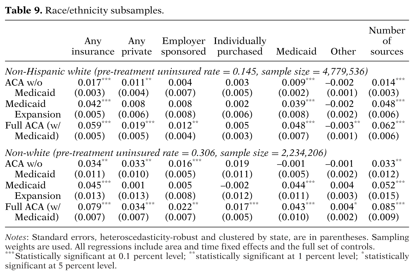
Table 9 reports results based on a stratification of our sample by race/ethnicity. We group individuals into two categories: non-Hispanic white or non-white. The pre-treatment uninsured rate among non-whites (30.6 percent) is roughly twice that for non-Hispanic whites (14.5 percent), so we expect bigger gains in coverage for non-whites. Our results support this hypothesis, as non-whites experience an estimated increase in coverage of 7.9 percentage points, whereas non-Hispanic whites experience an estimated 5.9 percentage point increase in coverage from full ACA implementation.

Table 8. Age subsamples

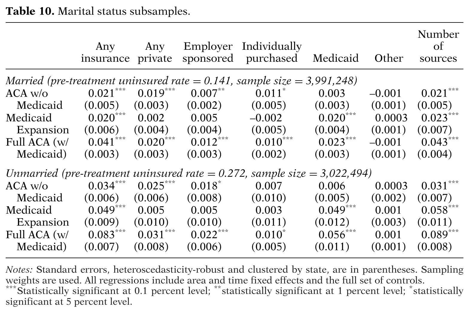
For both groups the increase in Medicaid coverage was larger than the increase in private insurance coverage. Table 10 presents the results of our marital status stratification analysis, which suggests larger gains in coverage among the unmarried. Full implementation of the ACA increased coverage by 8.3 percentage points (from a base of 72.8 percent) among the unmarried and by 4.1 percentage points (from a base of 85.9 percent) among the married. Among the married, full implementation of the ACA is predicted to increase Medicaid coverage by 2.3 percentage points and private insurance coverage by 2.0 percentage points (roughly split between increases in individually purchased insurance and ESI). Among the unmarried, full implementation of the ACA is predicted to increase Medicaid coverage by 5.6 percentage points and private insurance coverage by 3.1 percentage points (with about two-thirds of this increase coming from ESI).

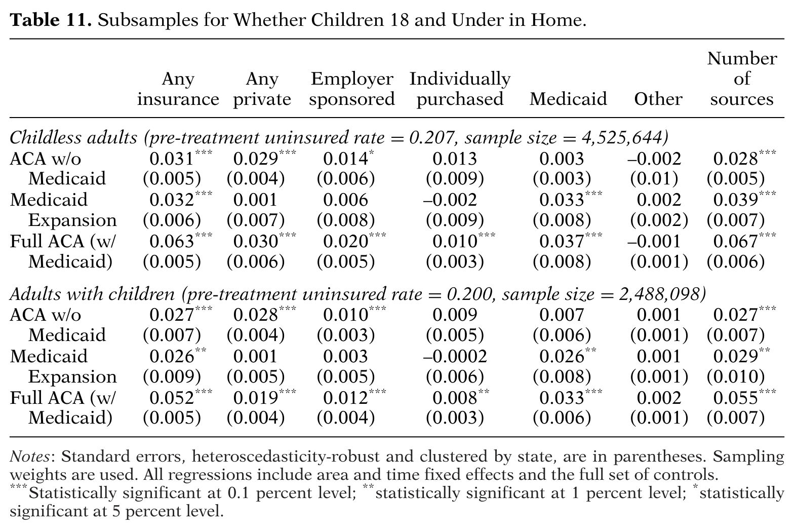
Table 11 shows the results dividing the sample based on whether individuals have children 18 years old or younger in the home. Prior to the ACA, most states had income eligibility cutoffs for Medicaid that were more stringent for childless adults than for adults with dependent children (or no categorical eligibility for childless adults), so we expect the ACA’s Medicaid expansion to have stronger effects for childless adults (McMorrow et al., 2016).

Table 9. Race/ethnicity subsamples

Table 10. Marital status subsamples

The results show that this is indeed the case, but only to a certain degree. Among childless adults, the full ACA increased overall coverage by 6.3 percentage points and Medicaid coverage by 3.7 percentage points. Among adults with children in the home, these effects were 5.2 and 3.3 percentage points, respectively.

Table 11. Subsamples for Whether Children 18 and Under in Home

Frean, Gruber, and Sommers (2016) also found that some of the Medicaid coverage gains among adults with children could be coming from those who were already eligible before the ACA (the “woodwork effect”).

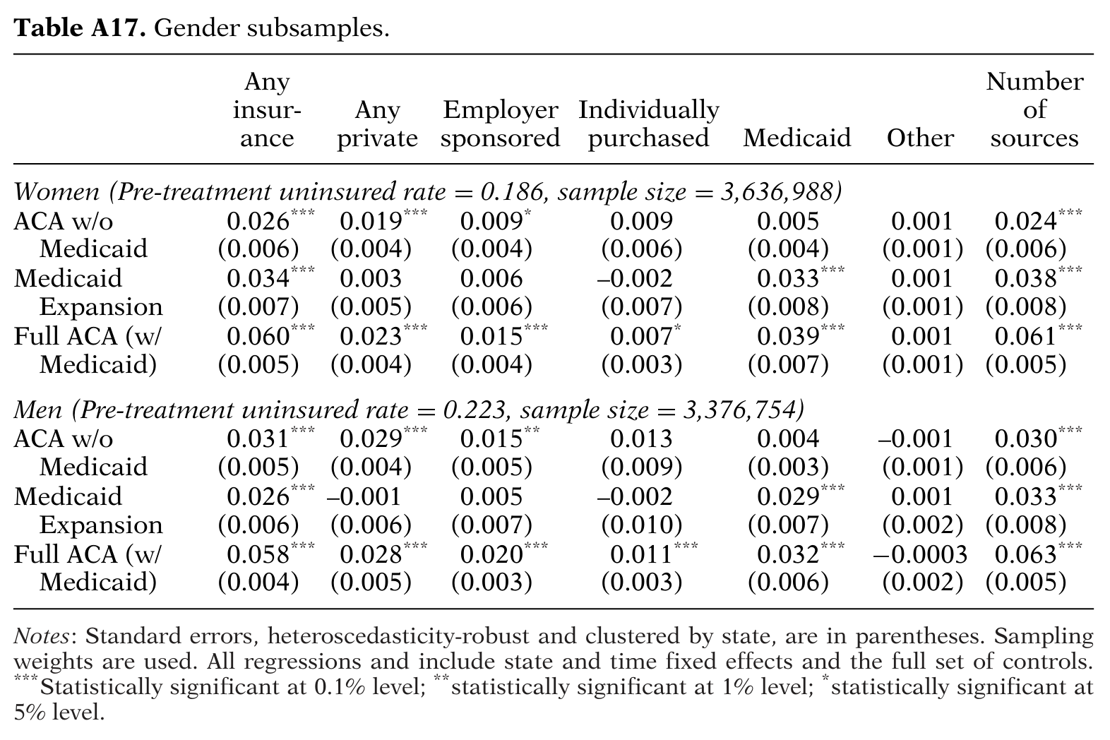
Our final subsample analysis stratifies the sample by gender. The estimated coverage gains are remarkably similar for both men and women. Given this similarity, we relegate the results table to Appendix Table A17.²⁹

DISCUSSION

Overall, our results suggest that, at the average local area pre-treatment uninsured rate, the Medicaid expansion component of the ACA increased coverage by 3.1 percentage points in 2014, while the implementation of the other components of the ACA increased coverage by 2.8 percentage points. Thus, fully implementing all of the 2014 provisions of the ACA is predicted to increase coverage by 5.9 percentage points. Since the 2013 non-elderly uninsured rate was 20.3 percent, our estimates imply that if the ACA had been fully implemented in all states, the non-elderly uninsured rate would have fallen by 29 percent. In contrast, the actual effect of the ACA—computed by taking the population-weighted average of the effects in Medicaid expansion and non-expansion states—has been just 22.77 percent.³⁰

These results for overall coverage alone extend the literature in several important ways. First, a simple comparison of the difference in coverage gains between Medicaid expansion and non-expansion states reported in the descriptive literature (Courtemanche, Marton, & Yelowitz, 2016; Long et al., 2014; Smith & Medalia, 2015) suggests an additional 1 to 1.5 percentage point coverage gain in expansion states in 2014. Our DDD results suggest that the causal impact of the Medicaid expansion at the mean pre-treatment uninsured rate is roughly two to three times as large as these descriptive estimates. Our DD specification produces a very similar estimated effect of the Medicaid expansion to these descriptive studies, and controlling for the interaction of the pre-treatment uninsured rate with the post-treatment indicator in the DDD model explains the difference in results. Similarly, we suspect that the simple pre–post comparisons from the descriptive literature also understate the effect of the Medicaid expansion because they do not account for the fact that, since non-expansion states had disproportionately high baseline uninsured rates, they likely would have experienced disproportionately high gains in coverage in the counterfactual where every state expanded Medicaid. This insight underscores the need for careful econometric designs when evaluating the impacts of the ACA’s Medicaid expansion in future research.

Second, our use of an alternative identification strategy allows us to separately estimate the causal impact of the Medicaid expansion and the casual impact of the other components of the ACA. Kaestner et al. (2015) and Wherry and Miller (2016) employed more rigorous econometric designs than the descriptive studies mentioned above to identify the coverage gains from the Medicaid expansion, but they did not aim to identify the causal effects of the collection of private insurance-related reforms that also took effect in 2014. We estimate that the effect of these reforms on the probability of having any form of coverage was roughly equal in magnitude (2.8 percentage points) to the impact of the Medicaid expansion (3.1 percentage points).

Third, we evaluate the impact of the ACA on a relatively detailed set of sources of insurance. Two of the descriptive studies we described, Long et al. (2014) and Smith and Medalia (2015), do not differentiate between different sources of coverage at all, while Kaestner et al. (2015) and Wherry and Miller (2016) only consider two sources of coverage, Medicaid and private coverage. We differentiate between private coverage coming from the employer-provided group market and that coming from the non-group market (such as exchange coverage) and discover they account for roughly equal shares of the increase in private coverage resulting from the ACA. This is a surprising and interesting result for two reasons. First, we might have expected a smaller effect on ESI, since the ACA deliberately did not try to alter the employer-provided market, and the employer mandate had not yet taken effect in 2014. One possible explanation is that the individual mandate may have increased take-up of ESI, either among employees or their spouses or dependents. Second, we might have expected a larger effect on individually purchased insurance since 8 million people enrolled in the exchanges in 2014 (U.S. Department of Health and Human Services, Office of the Assistant Secretary for Planning and Evaluation, 2014). Multiplying our results (1.1 percentage point increase in private coverage) by the number of U.S. residents (199 million; Colby & Ortman, 2015) in the 18 to 64 age range in 2014 and dividing by 8 million, we compute that only 27 percent of people who purchased a plan through the exchanges were newly covered. In other words, our results imply that most individuals in the exchanges in 2014 already had some form of insurance in 2013. This can be considered a form of crowd-out since most exchange plans were subsidized. Of course, even if those participating in the exchanges already had some sort of insurance prior to the ACA, the quality of their coverage may have improved with regard to deductibles, copayments, and range of services covered.

Another contribution of our paper is to present new results related to heterogeneity in the ACA’s impacts. We found that the coverage gains from the full ACA were largest for those without college degrees, non-whites, young adults, unmarried individuals, and those without children in the home. These results have important implications for disparities. For instance, our estimates imply that the fully implemented ACA reduced the difference in uninsured rates between the lowest (high school education or less) and highest (college graduate) education groups by 3.6 percentage points, or 11.4 percent.³¹ However, the ACA without the Medicaid expansion only lowered this gap by 6.7 percent.³² Similarly, the fully implemented ACA lowered the coverage disparity between whites and non-whites by 2.0 percentage points, or 14 percent, whereas the ACA without the Medicaid expansion actually increased this disparity.³³

Our education stratifications also contribute to the debate surrounding the potential for Medicaid to crowd-out private insurance among low-socioeconomic-status individuals. Similarly to Frean, Gruber, and Sommers (2016), we find no evidence that the Medicaid expansion crowded-out private coverage, either for the full sample or for any education subgroup. At first glance this result appears at odds with the Kaestner et al. (2015) finding of a larger crowd-out effect in their sample of adults with a high school degree or less, but their estimate was also statistically insignificant so we cannot conclusively say that their results differ meaningfully from ours.

Our final contribution is methodological: our identification strategy for the non-Medicaid expansion portion of the ACA can potentially be used in future research to identify the impacts of the ACA on other outcomes such as health care utilization, health, and personal finances. It should be noted, though, that identifying off of pre-treatment uninsured rates implicitly assumes that the extensive margin of coverage is the only pathway through which the ACA affects the outcome. We find this assumption reasonable in the context of health insurance coverage, but it may be more problematic for outcomes such as health care utilization and health. In these cases, other mechanisms such as the quality of coverage (intensive margin) and the income redistribution caused by the ACA’s subsidies and community rating might be expected to play a role as well, so the identification strategy would need to be adjusted accordingly.³⁴

An obvious caveat of our work is that, due to data availability, we only estimate the effects in the first year of full ACA implementation, 2014. As future waves of the ACS become available, it would be worthwhile to revisit our estimates. The number of people who purchased a plan through the ACA’s exchanges rose from 8 million in 2014 to 8.8 million in 2015, and 12.7 million have selected a Marketplace plan in 2016. The impacts on individually purchased coverage and overall coverage may therefore have become stronger over time, potentially due in part to considerable increases in the maximum size of the individual mandate penalty in both 2015 and 2016. In addition, the employer mandate had not yet taken effect in 2014 and several states (Pennsylvania, Indiana, Alaska, and Montana) have subsequently expanded their Medicaid program in 2015 or 2016. Though these subsequent policy changes may further increase coverage, higher than expected exchange premiums and insurer exits from the exchange market may have a dampening effect on coverage. Nonetheless, our paper provides important evidence about the ACA’s early effects that can help guide ongoing policy debates.

CHARLES COURTEMANCHE is an Associate Professor of Economics at the Andrew Young School of Policy Studies, Georgia State University, P.O. Box 3992, Atlanta, GA 30302. He is also a Research Associate for the National Bureau of Economic Research (NBER), and a Research Affiliate for the Institute for the Study of Labor (IZA, e-mail: ccourtemanche@gsu.edu). JAMES MARTON is an Associate Professor of Economics at the Andrew Young School of Policy Studies, Georgia State University, P.O. Box 3992, Atlanta, GA 30302 (e-mail: marton@gsu.edu).

BENJAMIN UKERT is a Postdoctoral Fellow at the Leonard Davis Institute of Health Economics at the University of Pennsylvania, 308 Colonial Penn Center, 3641 Locust Walk, Philadelphia, PA 19104 (e-mail: bukert@wharton.upenn.edu). AARON YELOWITZ is an Associate Professor of Economics at the Gatton School of Business and Economics, University of Kentucky, Lexington, KY 40506 (e-mail: aaron@uky.edu).

DANIELA ZAPATA is a Research Associate at IMPAQ International, 1101 Vermont Avenue, 11th Floor, Washington, DC 20005 (e-mail: zapata.daniela@gmail.com).

ACKNOWLEDGMENTS

We would like to thank three editors, four anonymous referees, Kitt Carpenter, Chad Cotti, Amanda Kowalski, and seminar participants at the 2015 Southern Economic Association Annual Meeting for their valuable comments. Any errors are, of course, our own.

References

• Abadie, A., Diamond, A., & Hainmueller, J. (2010). Synthetic control methods for comparative case studies: Estimating the effect of California’s tobacco control program. Journal of the American Statistical Association, 105, 493–505.
• Abadie, A., Diamond, A., & Hainmueller, J. (2011). SYNTH: Stata module to implement synthetic control methods for comparative case studies [Software item]. Retrieved June 1, 2016, from http://econpapers.repec.org/software/bocbocode/s457334.htm.
• Abraham, J. M., Karaca-Mandic, P., & Boudreaux, M. (2013). Sizing up the individual market for health insurance: A comparison of survey and administrative data sources. Medical Care Research and Review, 70, 418–433.
• Aizer, A. (2007). Public health insurance, program take-up, and child health. Review of Economics and Statistics, 89, 400–415.

• Akosa Antwi, Y., Moriya, A. S., & Simon, K. (2013). Effects of federal policy to insure young adults: Evidence from the 2010 Affordable Care Act dependent coverage mandate. American Economic Journal, 5, 1–28.

• Barbaresco, S., Courtemanche, C., & Qi, Y. (2015). Impacts of the Affordable Care Act dependent coverage provision on health-related outcomes of young adults. Journal of Health Economics, 40, 54–68.

• Benitez, J. A., Creel, L., & Jennings, J. (2016). Kentucky’s Medicaid expansion showing early promise on coverage and access to care. Health Affairs, 35, 528–534.
• Bertrand, M., Duflo, E., & Mullainathan, S. (2004). How much should we trust difference-in-differences estimates? Quarterly Journal of Economics, 119, 249–275.
• Blumberg, L. J., Garrett, B., & Holahan, J. (2016). Estimating the counterfactual: How many uninsured adults would there be today without the ACA? Inquiry, 53, 1–13.
• Buchmueller, T., Ham, J. C., & Shore-Sheppard, L. D. (2015). The Medicaid program. National Bureau of Economic Research, Working paper no. 21425.
• Cameron, A. C., & Miller, D. L. (2015). A practitioner’s guide to cluster-robust inference. Journal of Human Resources, 50, 317–372.
• Colby, S. L., & Ortman, J. M. (2015). U.S. Census Bureau, Current Population Reports, projections of the size and composition of the U.S. population: 2014 to 2060. Washington, DC: U.S. Government Printing Office. Retrieved June 1, 2016, from https://www.census.gov/content/dam/Census/library/publications/2015/demo/p251143.pdf.
• Courtemanche, C., & Zapata, D. (2014). Does universal coverage improve health? The Massachusetts experience. Journal of Policy Analysis and Management, 33, 36–69.
• Courtemanche, C., Marton, J., & Yelowitz, A. (2016). Who gained insurance coverage in 2014, the first year of full ACA implementation? Health Economics, 25, 778–784.
• Finkelstein, A. (2007). The aggregate effects of health insurance: Evidence from the introduction of Medicare. Quarterly Journal of Economics, 122, 1–37.
• Fitzpatrick, M. D. (2008). Starting school at four: The effect of universal pre-kindergarten on children’s academic achievement. B.E. Journal of Economic Analysis and Policy, 8, 1–40.
• Frean, M., Gruber, J., & Sommers, B. D. (2016). Premium subsidies, the mandate, and Medicaid expansion: Coverage effects of the Affordable Care Act. National Bureau of Economic Research, Working paper no. 22213.
• Golberstein, E., Gonzales, G., & Sommers, B. D. (2015). California’s early ACA expansion increased coverage and reduced out-of-pocket spending for the state’s low-income population. Health Affairs, 34, 1688–1694.
• Gruber, J. (2011). The impacts of the Affordable Care Act: How reasonable are the projections? National Bureau of Economic Research, Working paper no. 17168.
• Hu, L., Kaestner, R., Mazumder, B., Miller, S., & Wong, A. (2016). The effect of the Patient Protection and Affordable Care Act Medicaid expansions on financial well-being. National Bureau of Economic Research, Working Paper No. 22170.
• Kaestner, R. (2016). Did Massachusetts health care reform lower mortality? No, according to randomization inference. Statistics and Public Policy, 3, 1–6.
• Kaestner, R., Garrett, B., Gangopadhyaya, A., & Fleming, C. (2015). Effects of the ACA Medicaid expansion on health insurance coverage and labor supply. National Bureau of Economic Research, Working paper no. 21836.
• Kaiser Family Foundation (KFF). (2014). State decisions on health insurance marketplaces and the Medicaid expansion, 2014. Retrieved on November 1, 2015, from http://kff.org/health-reform/state-indicator/state-decisions-for-creating-health-insurance-exchanges-and-expanding-medicaid/.
• Kenney, G., Allison, R. A., Costich, J. F., Marton, J., & McFeeters, J. (2006). Effects of premium increases on enrollment in SCHIP: Findings from three states. Inquiry, 43, 378–392.
• Kowalski, A. (2014). The early impact of the Affordable Care Act state-by-state. National Bureau of Economic Research, Working paper no. 20597.

• Long, S. K., Stockley, K., & Yemane, A. (2009). Another look at the impacts of health reform in Massachusetts: Evidence using new data and a stronger model. American Economic Review, Papers & Proceedings, 99, 508–511.

• Long, S. K., Karpman, M., Shartzer, A., Wissoker, D., Kenney, G. M., Zucherman, S.,... Hempstead, K. (2014). Taking stock: Health insurance coverage under the ACA as of September 2014. Washington, DC: Urban Institute.

• Mach, A., & O’Hara, B. (2011). Do people really have multiple health insurance plans? Estimates of non-group health insurance in the American Community Survey. Social, Economic & Housing Statistics Division, Census Bureau, Working paper number 2011–28.
• Marton, J. (2007). The impact of the introduction of premiums into a SCHIP program. Journal of Policy Analysis and Management, 26, 237–255.
• Marton, J., & Yelowitz, A. (2015). Health insurance generosity and conditional coverage: Evidence from Medicaid managed care in Kentucky. Southern Economic Journal, 82, 535–555.
• Marton, J., Yelowitz, A., & Talbert, J. C. (2014). A tale of two cities? The heterogeneous impact of Medicaid managed care. Journal of Health Economics, 36, 47–68.
• Marton, J., Ketsche, P. G., Snyder, A., Adams, E. K., & Zhou, M. (2015). Estimating premium sensitivity for children’s public health insurance coverage: Selection but no death spiral. Health Services Research, 50, 579–598.
• Marton, J., Snyder, A., & Zhou, M. (2016). Enhanced citizenship verification and children’s Medicaid coverage. Economic Inquiry, 54, 1670–1683.
• Marton, J., Yelowitz, A., Talbert, J. C., & Shores, M. (2016). Does Medicaid managed care help equalize racial and ethnic disparities in utilization? Health Services Research, 51, 872–891.
• McMorrow, S., Kenney, G., Long, S. K., & Anderson, N. (2015). Uninsurance among young adults continues to decline, particularly in Medicaid expansion states. Health Affairs, 34, 616–620.
• McMorrow, S., Kenney, G., Long, S. K., & Goin, D. E. (2016). Medicaid expansions from 1997 to 2009 increased coverage and improved access and mental health outcomes for low-income parents. Health Services Research, 51, 1347–1367.
• Miller, S. (2012). The effect of insurance on emergency room visits: An analysis of the 2006 Massachusetts health reform. Journal of Public Economics, 96, 893–908.
• Mishra, A. N., Ketsche, P., Marton, J., Snyder, A., & McLaren, S. (2014). Examining the potential of information technology to improve public insurance application processes: Enrollee assessments from a concurrent mixed method analysis. Journal of the American Medical Informatics Association, 21, 1045–1052.
• Rosenbaum, P. R. (2002). Covariance adjustment in randomized experiments and observational studies. Statistical Science, 17, 286–327.
• Simon, K., Soni, A., & Cawley, J. (2016). The impact of health insurance on preventive care and health behaviors: Evidence from the 2014 ACA Medicaid expansions. National Bureau of Economic Research, Working paper no. 22265.
• Slusky, D. (2016). Significant placebo results in difference-in-differences analysis: The case of the ACA’s parental mandate. Eastern Economic Journal (forthcoming) http://link.springer.com/article/10.1057%2Feej.2015.49.

• Small, D. S., Ten Have, T. R., & Rosenbaum, P. R. (2008). Randomization inference in a group-randomized trial of treatments for depression: Covariate adjustment, noncompliance, and quantile effects. Journal of the American Statistical Association, 103, 271–279.

• Smith, J. C., & Medalia, C. (2015). U.S. Census Bureau, Current Population Reports, P60–253, health insurance coverage in the United States: 2014. Washington, DC: U.S. Government Printing Office.

• Sobel, R. S. (2014). The elephant in the room: Why some states are refusing to expand Medicaid. Applied Economics Letters, 21, 1226–1229.
• Sommers, B. D. (2010). Targeting in Medicaid: The costs and enrollment effects of Medicaid’s citizenship documentation requirement. Journal of Public Economics, 94, 174–182.
• Sommers, B. D., Buchmueller, T., Decker, S. L., Carey, C., & Kronick, R. (2013). The Affordable Care Act has led to significant gains in health insurance and access to care for young adults. Health Affairs, 32, 165–174.
• Sommers, B. D., Kenney, G. M., & Epstein, A. M. (2014). New evidence on the Affordable Care Act: Coverage impacts of early Medicaid expansions. Health Affairs, 33, 78–87.
• Sommers, B. D., Chua, K., Kenney, G. M., Long, S. K., & McMorrow, S. (2016). California’s early coverage expansion under the Affordable Care Act: A county-level analysis. Health Services Research, 51, 825–845.
• Sonier, J., Boudreaux, M., & Blewett, L. (2013). Medicaid “welcome-mat” effect of Affordable Care Act implementation could be substantial. Health Affairs, 32, 1319–1325.
• U.S. Department of Health and Human Services, Office of the Assistant Secretary for Planning and Evaluation. (2014). Health insurance marketplace: Summary enrollment report for the initial annual open enrollment period. Washington, DC: ASPE Issue Brief.
• Wherry, L. R., & Miller, S. (2016). Early coverage, access, utilization, and health effects associated with the Affordable Care Act Medicaid expansions: A quasi-experimental study. Annals of Internal Medicine, 164, 795–803.
• Wolfe, B., & Scrivner, S. (2005). The devil may be in the details: How the characteristics of SCHIP programs affect take-up. Journal of Policy Analysis and Management, 24, 499–522.

APPENDIX

Table A1. Pre-treatment summary statistics for control variables

Table A2. Predictors of state Medicaid expansion

Table A3. Predictors of baseline uninsured rates by state Medicaid expansion status

Table A4. Effect of ACA on probability of any private insurance with different sets of controls

Table A5. Implied effect of ACA on probability of any private insurance at mean pre-treatment uninsured rate: Other robustness checks

Table A6. Effect of ACA on probability of employer-provided insurance with different sets of controls

Table A7. Implied effect of ACA on probability of employer-provided insurance at mean pre-treatment uninsured rate: Other robustness checks

Table A8. Effect of ACA on probability of individually purchased insurance with different sets of controls

Table A9. Implied effect of ACA on probability of individually purchased insurance at mean pre-treatment uninsured rate: Other robustness checks

Table A10. Effect of ACA on probability of Medicaid with different sets of controls

Table A11. Implied effect of ACA on probability of having Medicaid at mean pre-treatment uninsured rate: Other robustness checks

Table A12. Effect of ACA on probability of other insurance with different sets of controls

Table A13. Implied effect of ACA on probability of having other insurance at mean pre-treatment uninsured rate: Other robustness checks

Table A14. Effect of ACA on number of sources of insurance coverage with different sets of controls

Table A15. Implied effect of ACA on number of sources of insurance coverage at mean pre-treatment uninsured rate: Other robustness checks

Table A16. Falsification tests

Table A17. Gender subsamples

Notes

1. There is also an employer mandate that will impose a financial penalty on employers with more than 50 employees that have at least one full-time employee who receives a premium tax credit. Implementation of this mandate was delayed until January 1, 2015, for businesses with more than 100 employees and January 1, 2016, for those with 50 to 99. More information is available at http://kff.org/interactive/implementation-timeline/.

2. In 2014, the penalty was the greater of (i) 1 percent of household income up to a maximum of the national average annual premium for a Bronze plan, or (ii) $95 per adult plus $47.50 per child up to a maximum of $285. The maximum increased to $975 in 2015 and $2,085 in 2016. See https://www.healthcare.gov/fees/fee-for-not-being-covered/.

3. See http://www.hhs.gov/healthcare/facts-and-features/key-features-of-aca-by-year/index.html#2014.

4. These other Medicaid policy changes include outreach (Aizer, 2007), application process changes (Mishra et al., 2014), waiting periods (Wolfe & Scrivner, 2005), premiums and other forms of cost sharing (Kenney et al., 2006; Marton, 2007; Marton et al., 2015), citizenship verification (Marton, Snyder, & Zhou, 2016; Sommers, 2010), and managed care implementation (Marton et al., 2014, 2016).

5. Some state-specific analyses also exist. Sommers, Kenney, and Epstein (2014) examine early Medicaid expansions in Minnesota, Connecticut, and Washington, DC. Sommers et al. (2016) and Golberstein, Gonzales, and Sommers (2015) examine the impact of California’s early expansion. Benitez, Creel, and Jennings (2016) document changes in coverage and access to care in Kentucky.

6. See http://data.bls.gov/timeseries/LNS14000000.

7. There are also a few new studies focusing on the impact of the Medicaid expansion on other outcomes, including financial well-being (Hu et al., 2016) and preventive care and health behaviors (Simon, Soni, & Cawley, 2016).

8. Kaestner et al. (2015) also employ synthetic control methods.

9. Blumberg, Garret, and Holahan (2016) construct a forecasting model to attempt to estimate how many individuals would have been uninsured in the absence of the ACA. We do not, however, consider this an attempt to estimate the causal effect of the full ACA since the forecast is based largely on an extrapolation from past trends.

10. The new 2010 Census boundaries generate 2,351 unique PUMAs, whereas the pre-2010 boundaries generated 2,071 unique PUMAs. These new boundaries are applicable to the 2013 ACS and beyond.

11. For each PUMA, both before and after the 2010 boundary change, we associated it with the CBSA that had the largest share of population within the PUMA. More than 99 percent of PUMAs map into at least one CBSA. Approximately 80 percent of PUMAs, containing 79 percent of the population, map into precisely one CBSA. Nearly 11 percent of PUMAs map into two CBSAs, with the remaining 8.5 percent mapping into three to six CBSAs.

12. According to tabulations from the 2013 ACS, 40 states had such a catch-all rural area. To examine the validity of grouping these rural areas within each state together, for each catch-all area we computed the range of the uninsured rate from the PUMAs from which they were constructed. On average, the uninsured rates varied by just 6.4 percentage points between the rural PUMAs with the lowest and highest uninsured rates within a state.

13. In lieu of the traditional Medicaid expansion, three states (Arkansas, Iowa, and Michigan) expanded with private coverage via a Section 1115 waiver. We attempted to test for differences between traditional and waiver expansions but were unable to draw clear conclusions given the small number of states choosing this option; we therefore simply classify the Section 1115 waiver states as being Medicaid expanders.

14. Most of these early expansions were relatively small, but Kaestner et al. (2015) consider five of them (Delaware; Washington, DC; Massachusetts; New York; and Vermont) to have been more complete. Even within these five states, though, the choice to expand Medicaid in 2014 still led to changes in Medicaid income eligibility limits for at least some eligibility categories.

15. We use state unemployment rates because the Bureau of Labor Statistics does not report unemployment rates at the CBSA level.

16. All appendices are available at the end of this article as it appears in JPAM online. Go to the publisher’s website and use the search engine to locate the article at http://onlinelibrary.wiley.com.

17. Note that we do not need to separately include $MEDICAI{D}_s$ in the model since it would be perfectly collinear with the local area fixed effects (recall that local areas are nested within states); our results are very similar if we drop the area fixed effects and include $MEDICAI{D}_s$ instead.

18. All appendices are available at the end of this article as it appears in JPAM online. Go to the publisher’s website and use the search engine to locate the article at http://onlinelibrary.wiley.com.

19. Local area pre-ACA uninsured rates reach as low as 3 percent in our data, so we do observe areas that are close to the hypothetical 0 percent. We experimented with non-linear functional forms (e.g., quadratic, including a series of dummy variables) for the uninsured rate and found that they do not reveal any meaningful new information.

20. Not considering our estimate of ${\gamma }_2$ to be interpretable as a causal effect is consistent with the interpretation used by Miller (2012) in her study that used a pre-treatment uninsured rate-based strategy to estimate the effects of the Massachusetts health care reform.

21. All appendices are available at the end of this article as it appears in JPAM online. Go to the publisher’s website and use the search engine to locate the article at http://onlinelibrary.wiley.com.

22. We implement the synthetic control method using the STATA module “synth” (Abadie, Diamond, & Hainmueller, 2011).

23. We have also computed the average effects across all individuals in the sample and found them to be very similar to the effects at the mean. We therefore do not report both numbers. We estimate the standard errors of these implied effects using the “lincom” command in Stata: http://www.stata.com/manuals13/rlincom.pdf.

24. For the “Stratify by Medicaid Expansion Status” column, the result reported in the “ACA without Medicaid expansion” row is from the DD regression for non-expansion states while the result in the “Full ACA” row is the corresponding estimate from the regression for expansion states. The top sample size is from the regression for non-expansion states and the bottom sample size is from the regression for expansion states.

25. All appendices are available at the end of this article as it appears in JPAM online. Go to the publisher’s website and use the search engine to locate the article at http://onlinelibrary.wiley.com.

26. Sonier, Boudreaux, and Blewett (2013) discuss the potential for this “woodwork” or “welcome-mat” effect. Marton and Yelowitz (2015) highlight that non-participating eligibles may view themselves as “conditionally covered” and the individual mandate then compels such participation.

27. Online appendix Tables A4 through A15 show that our sources of coverage results remain broadly similar across the various robustness checks. All appendices are available at the end of this article as it appears in JPAM online. Go to the publisher’s website and use the search engine to locate the article at http://onlinelibrary.wiley.com.

28. All appendices are available at the end of this article as it appears in JPAM online. Go to the publisher’s website and use the search engine to locate the article at http://onlinelibrary.wiley.com.

29. All appendices are available at the end of this article as it appears in JPAM online. Go to the publisher’s website and use the search engine to locate the article at http://onlinelibrary.wiley.com.

30. 54.35 percent of our sample lives in states that expanded Medicaid while 45.65 percent lived in non-expansion states. The weighted average effect is therefore 5.9 percentage points × 54.35 percent + 3.1 percentage points × 45.65 percent, which comes to 4.62 percentage points, or 22.77 percent of the 20.3 percent baseline uninsured rate.

31. These calculations are based on the results from Table 7. The 2013 uninsured rates for the lowest and highest education groups were 31.5 and 8.1 percent, respectively, for a difference of 23.4 percentage points. The full ACA increased insurance coverage for these two groups by 6.3 and 2.7 percentage points, respectively, reducing this difference by 3.6 percentage points, or 11.4 percent of 31.5.

32. This calculation is based on the same process discussed in the previous footnote, but replacing the 6.3 and 2.7 percentage point effects from the full ACA with the 4.2 and 2.1 percentage point effects among the lowest and highest education groups from the ACA without the Medicaid expansion.

33. These calculations are based on the results from Table 9. The 2013 uninsured rates for non-whites and whites were 30.6 and 14.5 percent, for a difference of 16.1 percentage points. Subtracting the estimated effects of the full ACA for the two groups reduces this difference to 14.1 percentage points, for a 2.0 percentage point reduction, which represents 14 percent of 16.1.

34. The ACA could affect health insurance rates through its effects on employers. Kaestner et al. (2015) find small effects of the ACA Medicaid expansion on labor supply, suggesting that such spillovers would not be large.