We assess the effect of a means- and asset-tested social insurance program, Medicaid, on the savings behavior of households. We do so using data on both asset holdings and consumption, matched to information on the eligibility of families for health insurance coverage under this program. Exogenous variation in Medicaid eligibility is provided by the dramatic expansion of this program over the 1984–93 period. We document that Medicaid eligibility has a sizable and significant negative effect on wealth holdings, and we confirm this finding by showing a strong positive association between Medicaid eligibility and consumption expenditures. We also exploit the fact that asset testing was phased out by the Medicaid program over this period to document that these Medicaid effects are much stronger in the presence of an asset test.
Recommended citation
Jonathan Gruber and Aaron Yelowitz. “Public Health Insurance and Private Savings.” Journal of Political Economy 107(6) (1999): 1249–1274. https://doi.org/10.1086/250096
Jonathan Gruber and Aaron Yelowitz. “Public Health Insurance and Private Savings.” Journal of Political Economy 107(6) (1999): 1249–1274. https://doi.org/10.1086/250096
Complete article reading edition. Tables and figures reproduce the published source; open an image for full resolution. The PDF retains the original page layout.
Abstract
We assess the effect of a means- and asset-tested social insurance program, Medicaid, on the savings behavior of households. We do so using data on both asset holdings and consumption, matched to information on the eligibility of families for health insurance coverage under this program. Exogenous variation in Medicaid eligibility is provided by the dramatic expansion of this program over the 1984–93 period. We document that Medicaid eligibility has a sizable and significant negative effect on wealth holdings, and we confirm this finding by showing a strong positive association between Medicaid eligibility and consumption expenditures. We also exploit the fact that asset testing was phased out by the Medicaid program over this period to document that these Medicaid effects are much stronger in the presence of an asset test.
Author affiliations
Jonathan Gruber — Massachusetts Institute of Technology and National Bureau of Economic Research
Aaron Yelowitz — University of California, Los Angeles and National Bureau of Economic Research
Acknowledgments
We are grateful to Peter Diamond, Robert Lucas, Annamaria Lusardi, Jonathan Skinner, Guglielmo Weber, two anonymous referees, and numerous seminar participants for helpful comments and to the National Institute on Aging (Gruber and Yelowitz) and the National Science Foundation (Gruber) for financial support.
I. Introduction
One of the most striking regularities about savings behavior in the United States is the skewed nature of wealth holdings: the median asset/income ratio for households headed by a 35—44-year-old high school dropout is one-tenth that of households headed by a 35—44-year-old college graduate.1 In a provocative recent article, Hubbard, Skinner, and Zeldes (1995) suggest that one explanation for this skewness is the structure of means-tested social insurance programs for lower-income households in the United States, which both mitigate the need for precautionary savings through the provision of a welfare safety net for consumption and tax away individual savings through means testing of assets to qualify for government assistance.
While compelling in theory, however, the practical importance of social insurance programs for savings behavior at the bottom of the income distribution is not clear; there is little evidence on the response of the savings or consumption decisions of low-income households to means-tested, asset-tested social insurance programs.
This paper assesses the savings impacts of one major social insurance program, Medicaid, which provides health insurance for low-income individuals. By providing first-dollar coverage of medical expenditures for qualifying individuals, Medicaid substantially lowers the expenditure risk facing both uninsured families and those privately insured families that drop plans with large copayments or deductibles to join the free Medicaid program. Moreover, along with means testing, Medicaid has also traditionally incorporated asset tests into its eligibility determination process. If social insurance is playing the role suggested by the Hubbard et al. model, savings and consumption should respond to programs such as Medicaid.
During the late 1980s and early 1990s, the Medicaid program substantially eased its eligibility criteria over this period, first by state fiat and later by federal mandate. The expansion occurred at a differential pace across the states, and even within states through differential age cutoffs for the eligibility of children. This quasi randomization of insurance coverage allows us to assess the effect of providing free health insurance on savings behavior while avoiding issues of selection in who chooses public insurance coverage. Moreover, throughout this period, states were removing their asset tests for program qualification. This allows us to quantify the interaction between means testing and asset testing of eligibility for this program.
To carry out this test, we use data from two sources. The first is the Survey of Income and Program Participation (SIPP), the largest nationally representative survey with annual data on the asset holdings of the U.S. population. The second is the Consumer Expenditure Survey (CEX), the only U.S. database with annual data on total family consumption levels. We construct a household-specific valuation of the Medicaid expansions and match this measure to the SIPP data on household asset holdings and the CEX data on consumption. We find a highly significant, negative relationship between the generosity of a family’s public insurance entitlement and that family’s asset holdings. We confirm this finding by showing that there is a strong positive effect of Medicaid entitlement on consumption spending. And, in both cases, we find that the effect of Medicaid eligibility is much stronger in the presence of an asset test. The robustness of our finding across two very different sources of data confirms that Medicaid is an important determinant of the savings decisions of eligible households.
Our paper proceeds as follows. In Section II, we provide some theoretical background, review previous evidence on social insurance and savings, and describe the Medicaid expansions that form the backbone of our empirical approach. In Section III, we discuss the data and estimation strategy. Section IV presents our SIPP results for asset accumulation and our CEX results for consumption. Section V presents conclusions.
II. Background
The Medicaid Expansions
Medicaid coverage of medical expenses was traditionally limited primarily to very low income, single female—headed families that received cash welfare under the Aid to Families with Dependent Children (AFDC) program. Beginning in 1984, however, the program expanded eligibility for all children and for pregnant women; that is, for women, these expansions applied to the expenses of pregnancy only. From 1984 to 1987, there were increases in Medicaid eligibility for very poor families that did not meet the eligibility criterion because of family structure (these changes expanded on similar state programs that existed before 1984). From 1987 onward, there were substantial increases in the income cutoff for Medicaid eligibility for children and pregnant women in all family structures. By 1990, states were required to cover all pregnant women and children under the age of 6 up to 133 percent of poverty (independent of family composition) and were allowed to expand coverage up to 185 percent of poverty.2 In addition, children born after September 30, 1983, were mandatorily covered up to 100 percent of poverty (once again independent of family composition). These expansions are described in more detail in Currie and Gruber (1996a, 19960). Nationally, the expansions had an enormous impact on the Medicaid eligibility of children and pregnant women: by 1992, roughly one-third of the children in the United States were eligible for Medicaid for coverage of their medical expenses, and almost one-half of the women were eligible for the expenses of pregnancy.
While most of the legislative action over this period occurred at the federal level, there was tremendous heterogeneity in the impacts of Medicaid policy changes across the states. States initially had dif ferent qualification limits through AFDC and other optional programs, so that the uniform national expansions had differential impacts. In addition, states took up the new eligibility options at different rates, providing variation in the timing of the expansions as well as the ultimate size of their effects. There was also variation within states in the eligibility of children of different ages for the Medicaid expansions due to different age thresholds in the laws.
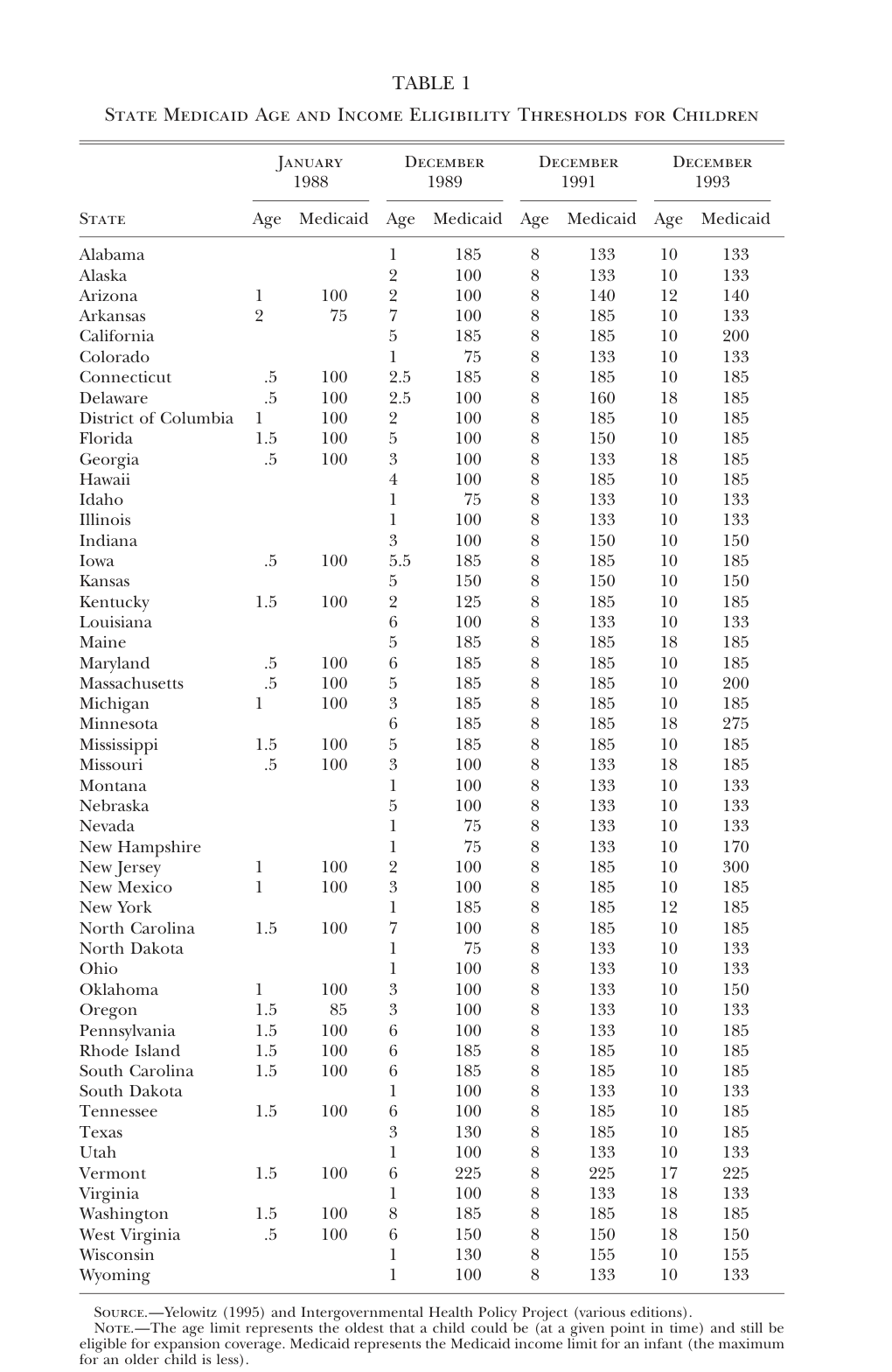
Table 1, updated from Yelowitz (1995), illustrates this variation by showing the age and percentage of poverty cutoffs for expansions to the youngest group of children in each state at four different points in time.3 In January 1988, only some states had expanded eligibility, and the income and age cutoffs varied. By December 1989, all states had some expansion in place since federal law mandated coverage of infants up to 75 percent of the poverty line; but some states had expanded coverage up to age 7 or 8, and coverage ranged as high as 185 percent of the poverty line. By December 1991, state policies were more uniform as the most restrictive federal mandates had taken place, but some variation in poverty cutoffs remained. In the subsequent years, several states expanded the age limits even further, using only state funds.
A key feature of these expansions is that the population that was affected was not just the uninsured, but also those with private insurance. Indeed, as Cutler and Gruber (1996) note, two-thirds of those made eligible for the Medicaid expansions were already covered by private insurance before becoming eligible. This raises the prospect that the expansion of the Medicaid program may have ‘‘crowded out’ purchases of private insurance, a claim that has found empirical support in a series of papers over the past several years (Currie 1995; Rask and Rask 1995; Cutler and Gruber 1996).4 But no previous studies have explored another potentially interesting avenue of crowd-out: reduced asset accumulation in response to increases in Medicaid eligibility.
Table 1. STATE MEDICAID AGE AND INCOME ELIGIBILITY THRESHOLDS FOR CHILDREN
Notes: SourcE.—Yelowitz (1995) and Intergovernmental Health Policy Project (various editions).
Notes: Nore.—The age limit represents the oldest that a child could be (at a given point in time) and still be eligible for expansion coverage. Medicaid represents the Medicaid income limit for an infant (the maximum for an older child is less).
Theoretical Background
There are three channels through which increased Medicaid generosity might affect savings and consumption decisions: precautionary accumulation, redistribution, and asset testing. First, by reducing medical expenditure risk for eligible families, the Medicaid program lowers their need for precautionary savings. This will raise consumption and lower wealth holdings.5 This point is explicitly demonstrated by Kotlikoff (1989). He presents simulations of a life cycle model with uncertainty that demonstrate that asset accumulation will be much lower in an economy with public insurance available than in one in which individuals self-insure their medical expenses through savings.6
Of course, this effect will operate only to the extent to which eligible (low-income) families are using savings as self-insurance against medical risk. Self-insurance of medical expenses, despite their high variability, may be a reasonable option for many families. Unless a family has access to a large group through which to purchase insurance, health insurance can be prohibitively expensive, and non— group policies often come with severe limitations on benefits that further reduce their value. There may also be some self-insurance of medical spending risk among the insured who (potentially) move onto the Medicaid program as well. The average privately insured family pays about one-third of its medical costs (Cutler and Gruber 1996). These costs are to some extent variable (up to plan out-of-pocket maxima), so that families that do not typically hit the out-of-pocket maximum may be saving as insurance against a particularly expensive year of medical spending. In contrast, Medicaid provides first-dollar coverage of virtually all medical expenses. Thus, when a privately insured family moves onto Medicaid, its (limited) precautionary savings may be reduced. This negative effect on wealth holdings is offset, however, by the second effect: Medicaid is explicitly redistributive and as such increases the resources of persons who become eligible for the program. For those who were previously uninsured, this increase occurs through reducing their expected medical outlays. For those who have private insurance but choose to drop it in order to sign up for the Medicaid program, there is a reduction in expected outlays for both out-of-pocket spending and insurance payments.7 This redistributive transfer is transitory: it lasts only as long as the family is eligible for Medicaid, on both income and demographic grounds.
Thus, to the extent that families are operating in a forward-looking life cycle framework, the transfer will be saved and spread over future periods in which there is higher risk of out-of-pocket medical expenses, offsetting the precautionary savings effect.
On the other hand, to the extent that families are not perfectly forward-looking, some of this transfer will be spent today. Moreover, if the family is qualifying for Medicaid because it is transitorily poor, then the transfer will also be spent. In this case, the increase in savings from this transfer will be smaller; in the limit, there may be no change in savings, and it will all be spent today. Thus the net effect of expanded Medicaid on wealth accumulation is ambiguous. On the other hand, the effect on consumption is unambiguous: it will increase through reduced precautionary accumulation, as well as (to some extent) through increased spending in response to this redistributive transfer.
The third and final channel is one that is highlighted by Hubbard et al. (1995): asset testing. Traditionally, eligibility for AFDC (and hence Medicaid) was conditioned on asset holdings of less than $1,000 per family.8 As part of the legislation that allowed states to expand their income cutoffs for Medicaid eligibility, the federal government also authorized states to remove their asset tests for determining eligibility. States were quick to drop asset testing once they had the chance, so that by the middle of 1989, fewer than 10 states still had asset tests. Over the entire population, asset tests should lower savings; but this effect might be expected to be small, to the extent that a large share of the population does not consider Medicaid to be a relevant option. Of more interest for our purposes is the interaction of asset tests with eligibility. On the one hand, following the logic of Hubbard et al., in a world with an asset test, individuals who are made eligible on income grounds but not on asset grounds may reduce their savings to qualify for the program. In this case the presence of an asset test will exacerbate the savings reduction (and consumption increase) from expanding Medicaid since the newly eligible individuals must reduce their savings to qualify (on top of the precautionary effect discussed earlier).
On the other hand, if an asset test is in place, newly eligible individuals with reasonably high savings may not consider this program a realistic option, so that the expansions will not affect their savings.
Under this model, asset tests may mitigate the savings and consumption effects of expansions since there is no precautionary savings effect or redistributive effect for newly eligible persons who are high savers (and who consider the program irrelevant). Finally, asset tests may have no effect in that they are not binding or difficult to enforce. Thus the net interactive effect of asset tests and eligibility is unclear. As a result, on net across these three effects, there is an ambiguous prediction for the effect of Medicaid eligibility on savyings, but an unambiguous prediction that Medicaid eligibility should raise consumption.
Related Empirical Work
Precaution is clearly an important motivation for savings; more households report precautionary saving as an important motive for their saving than any other reason (Kennickell and Starr-McCluer 1994). In addition, a series of tests assessing the effects of variation in income risk across families on savings show that more risk leads to lower consumption and larger asset holdings (see, e.g., Dardanoni 1991; Guiso, Jappelli, and Terlizzese 1992; Dynan 1993; Browning and Lusardi 1996; Kazarosian 1997; Carroll and Samwick 1998). As Engen and Gruber (1995) discuss, however, these tests suffer from the problem that individual income risk may be the result of factors that also determine savings, such as preferences for risk; moreover, even if precaution is an important motivation for savings on average, one cannot naturally assume that social insurance programs crowd out this precautionary savings on the margin.
There is previous empirical evidence on the effects of three different social insurance programs on savings. Kantor and Fishback (1996) explore the impact of the introduction of insurance against workplace injuries under the workers’ compensation program and find that there was a 25 percent reduction in the savings of working households. Engen and Gruber (1995) estimate the relationship between the generosity of the unemployment insurance program and wealth holdings, and find that increasing the generosity of unemployment insurance by one-half would lower savings by 14 percent.
Finally, there is a large literature on the effect of the Social Security program on savings: time-series estimates of the effect of Social Security vary (Feldstein 1974, 1982; Leimer and Lesnoy 1982), and individual-level estimates indicate that each dollar of Social Security wealth is translated to 45 cents less in savings (Diamond and Hausman 1984).
These previous studies may not be predictive of the effect of Medicaid, however, for four reasons. First, although the benefit structure of each of these programs is progressive, none of the programs are means tested. Second, for the first two programs, under the empirically supported assumption that the costs of these social insurance benefits were fully shifted to workers’ wages,9 there is no redistributive effect of the type described above. Third, none of these programs are asset tested. Finally, in these other cases, private insurance coverage is rare.10 But 71 percent of the nonelderly population is covered by private health insurance in the United States (Employee Benefits Research Institute 1996). Thus those individuals who remain uninsured may be a selected sample with little risk of medical spending (or a low level of risk aversion), so that there is little precautionary saving to be crowded out among the uninsured.
The only paper of which we are aware that explicitly estimates the effects of asset tests is Powers (1998). She examines the effect of variations in asset testing for the AFDC program in the 1970s on the savings of single female—headed households. She finds a very strong effect of asset tests: each one-dollar rise in the asset limit raises the savings of this population by 50 cents. But this study does not explore the role of program generosity, nor the interaction of generosity with asset testing.
Another closely related study is the paper by Starr-McCluer (1996), who studies the correlation between wealth holdings and insurance coverage. An important problem with this approach, however, is that insurance status is an outcome of the same choice process that determines savings decisions. Perhaps as a result, Starr-McCluer finds a positive effect of insurance coverage on wealth holdings. Thus the effect of health insurance on precautionary savings remains an open question, which we can address with our plausibly more exogenous variation in Medicaid eligibility.
III. Empirical Strategy
Data
Our data come from two sources. The first is the Survey of Income and Program Participation, covering the years 1984-93. A new SIPP panel is introduced each calendar year, follows individuals for 24–32 months, and surveys approximately 15,000-—20,000 households.
Because the panels overlap, households from as many as three different panels may be observed at a given point in time. Each panel interviews individuals in four-month intervals known as waves, where the respondent is asked retrospective information about income, labor force activity, and participation status in public programs over the preceding four months.
The other major element of the SIPP is the various ‘‘topical modules” that are included during selected household visits. One of these supplements provides information on household wealth holdings. These questions are asked once or twice per panel, usually one year apart. This regular source of data on wealth holdings, collected for a large nationally representative sample over the period of the Medicaid expansions, makes the SIPP the best data source for our purposes. The wealth inventory is available for the fourth and seventh waves of 1984-86, the fourth wave of 1987, 1990, and 1992, and the seventh wave of 1991.11
Our unit of observation in the SIPP sample is the household; since the wealth summary measures are collected only at the household level, we excluded households with more than one family in residence. Our sample consists of all households that were present in the SIPP at the point of the wealth interview, in which the head is between the ages of 18 and 64, and in which there are no household members over the age of 64, so that we can avoid complications aris ing from public insurance provided to those aged 65 and over by the Medicare program. And we consider only households that live in a State that is uniquely identified by the SIPP, which groups some of the smaller states.
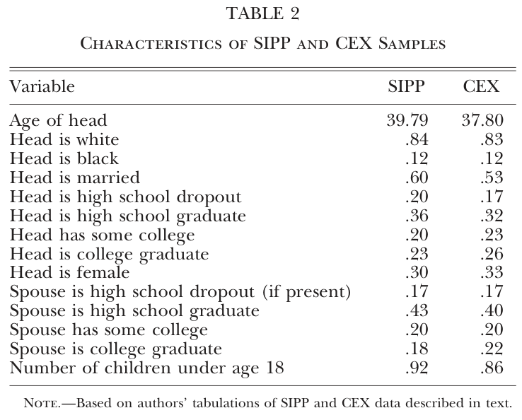
Notes: Note.—Based on authors’ tabulations of SIPP and CEX data described in text.
Wealth is measured as total household net worth, which is the sum of financial assets, home equity, vehicle equity, and business equity, net of unsecured debt holdings. Roughly one-quarter of the households in our data set have imputed wealth information. The SIPP imputation methodology has been criticized by a number of commentators (Curtin, Juster, and Morgan 1989; Hoynes, Hurd, and Chand 1995). We therefore exclude imputed values for our analysis.
Table 2 presents summary statistics of selected covariates for the head of the household and the head’s spouse (if present). Our second data set is the Consumer Expenditure Survey. We use CEX data for the 1983-93 period. The CEX collects information on a complete inventory of consumption items for a rotating sample of households each year. Households are interviewed for up to four quarters, providing information on household characteristics and consumption of different categories of goods. We use total nondurable, nonmedical consumption as our dependent variable for part of the CEX analysis.12 Our CEX variables are averaged over all the interviews for which the household is present. The CEX sample se lection criteria are the same as for the SIPP; fewer states are identified in the CEX, however, because of confidentiality restrictions. The means of this data set are provided in table 2 as well. The CEX and SIPP samples are very similar: the CEX sample is somewhat younger and less likely to be married and has smaller families.
Construction of a Medicaid Variable
The impact of Medicaid on household savings decisions will be determined by the magnitude of the associated reduction in medical expenditure risk for that household. We therefore define the generosity of the Medicaid program for a given household as the amount of expected medical spending that is made eligible for the Medicaid program, which we call ‘“‘Medicaid eligible dollars.’’ This measure of generosity varies across households for three reasons. The first is the legislative environment, which determines the types of individuals eligible for Medicaid (i.e., age ranges of eligibility for children) and the income level. The second is household characteristics, both those that determine eligibility (such as income) and those that determine the value of being eligible. Since
(e.g.) a newborn is more medically costly than a 10-year-old, family structure determines how much medical spending will be made eligible for the family under a given legislative environment. And the third is the cost of medical care in the area. This measure provides a natural parameterization of the effects of the Medicaid program on the household unit as a whole, which should determine savings decisions.13
More precisely, we proceed as follows. First, for each child and each woman of childbearing age, we assign a likelihood of being Medicaid eligible, based on their characteristics, using a detailed simulation model of Medicaid eligibility described in Currie and Gruber (1996a, 19965). We denote each individual’s eligibility by ELIG;. Second, we proxy the benefits of making a person of a given age and sex eligible for Medicaid by the mean spending of persons of that age and sex. We compute age /sex-specific spending on medical care from the 1987 National Medical Expenditure Survey (NMES) for 22 age/sex groups; these data are reported in the appendix to Cutler and Gruber (1996). Third, we normalize these national average spending figures by an index of relative state-specific medical costs, formed by taking the Medicaid expenditure for one AFDC adult and two AFDC children in each state (except Arizona, which had a Medicaid demonstration project) for the years 1984–93, deflating to 1987 dollars, averaging over the 10 years, and normalizing to one in the median state. The index varies from 0.70 in Mississippi to 1.38 in New York (there is one outlier state—Alaska— with a value of 1.77). We denote the area-specific, age-specific, spending measure as .14
We combine these two components of generosity to form Medicaid eligible dollars:
Equation (1):
where is the expected dollars of medical spending that are made eligible for family , which consists of individuals . As Medicaid becomes more generous, either by increasing its income cutoffs or by covering more expensive family members, MED rises. We measure this value at each of the waves that precedes and includes the wealth wave in the SIPP and at each quarterly interview in the CEX, and we use the average in our regression. In this way, we smooth any noise in the measurement of family structure.
One practical problem with this approach, however, is that income is endogenous to the savings/consumption decision: income depends directly on savings through capital income receipt; labor supply may be changing as a result of efforts to qualify for Medicaid; and changes in private insurance coverage that result from becoming eligible may be reflected in wages (to the extent that the employer costs of insurance are shifted to wages) as well as in savings.
As a result, we actually estimate our models by instrumental variables, where the instrument SIMMED_j is defined as
Equation (1′):
The variable SIMELIG is formed by imputing to each potentially eligible woman or child a likelihood of Medicaid receipt that is based only on purely exogenous characteristics that are correlated with their eligibility: the education of the household head (for children) or of the woman, the age of the child, state of residence, and year.
The last three of these criteria are directly related to the dimensions of legislative variation in Medicaid policy. The first, education, serves as an exogenous proxy for income. We use four education categories: less than high school, high school graduate, some college, and college graduate.
Our imputation strategy is to measure the average eligibility rate in a given education/age/state/year cell, using data from the March Current Population Survey (CPS), and then to assign that average eligibility to all persons in that cell in both the SIPP and CEX.15 We first select from the CPS for each year a national random sample of children of each age and of women of childbearing age, in each of the four education categories. We then compute the eligibility of each person in this same sample, for each state’s rules in that year. We then measure the average eligibility in each education /age/state cell to get a cell-specific eligibility measure. By using a nationally representative sample instead of a state-specific sample, we avoid any problems of correlations between state-specific demographic characteristics that determine eligibility and the savings / consumption behavior of residents of that state. In essence, this is a convenient parameterization of the rules of each state, as applied to the typical person in an education/age group cell.16
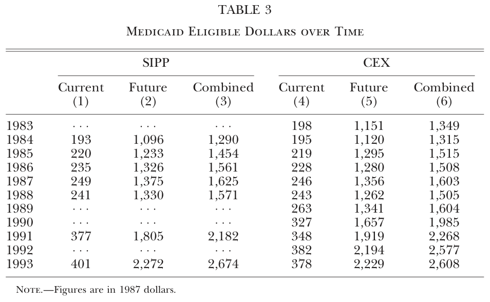
The time trends in (simulated) Medicaid eligible dollars for our SIPP and CEX samples are shown in columns | and 4 of table 3. The pattern is very similar across the two data sets: Medicaid eligible dollars roughly double over the 1984-93 period. Our CEX sample starts one year earlier, as noted above. There are no SIPP data for the years 1989, 1990, and 1992 since there was no survey in 1988 or 1989, and both the 1990 and 1991 wealth interviews took place during 1992.
Current eligibility for Medicaid is not the sole determinant of savings and consumption decisions, however: what is relevant is the entire future path of Medicaid eligibility. That is, consider two families that are living at the poverty line, in a state that has just expanded eligibility for children under age 6 to 133 percent of poverty. The first family has one child who is age 5, and the second has one child who is age 1. The effect on the savings and consumption of the second family will be much larger than on those of the first family since they face more years of reduced risk of medical expenditure.
We therefore also create a measure of expected future Medicaid eligible dollars (both actual and, as an instrument, simulated). For projecting future eligibility, we assume static expectations over the evolution of Medicaid policy; that is, we assume that individuals assess the eligibility of their family members if today’s law remains in place into the infinite future. The family traces out the eligibility of a given family member as that member ages, within the constraints of today’s eligibility of children of different ages (and pregnant women). We then discount future Medicaid eligibility dollars back to the present at a real interest rate of 6 percent.
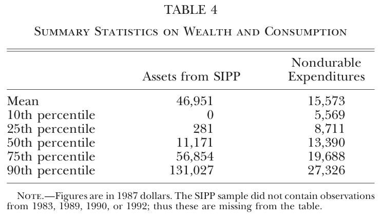
Table 4. SUMMARY STATISTICS ON WEALTH AND CONSUMPTION
Notes: Nore.—Figures are in 1987 dollars. The SIPP sample did not contain observations from 1983, 1989, 1990, or 1992; thus these are missing from the table.
Overall, Medicaid makes much more spending eligible in the future than it does today, as shown in table 3. The amount of future Medicaid dollars eligible is roughly five times the amount of current dollars eligible, although the time pattern is similar. Once again, the time patterns across the SIPP and CEX samples are very close. In our basic regression formulation, our Medicaid eligible dollars regressor (and instrument) is the sum of current dollars eligible (over the past year) and future dollars eligible, as shown in columns 3 and 6 of table 3.
Regression Specification
Our basic regression specification is
Equation (2):
where is household net worth or consumption, is the sum of current and future Medicaid eligible dollars, is the education categories used to match Medicaid eligibility, is a set of controls for family demographic structure, is an additional set of household-level covariates, is a full set of state dummies, and is a full set of time dummies.
Our dependent variable for this analysis is a measure of household total net worth, or consumption in the CEX. Wealth holdings are very skewed, as we show in table 4: 23 percent of our sample has net worth of less than or equal to zero; the median net worth in our sample is $11,171, and the mean is $46,951.17 As a result, we use the log of wealth (or consumption) as our dependent variable. This raises the problem, however, that there may be sample selection bias to estimates based solely on positive wealth observations. In fact, as we show below, there is a significant relationship between Medicaid eligibility and positive wealth holdings. But we argue that the size of this relationship cannot explain much of the very large crowd-out that we find in our log wealth models. Moreover, sample selection is not a problem for our consumption models since there are no observations with zero consumption. Thus the confirmation of our basic conclusions in the consumption data illustrates that our wealth results are not driven by selection. We estimate this model by instrumental variables, where the instrument is SIMMED,. The first-stage fit is excellent: the /statistic on the excluded instrument is over 7,000.
Our instrumented regressor, Medicaid eligible dollars, varies along four dimensions: education, state, year, and family structure (age and number of children and age of woman). Each of these dimensions may be independently correlated with savings decisions.
As a result, we include controls for each: dummies for each educational category;18 dummies for each state; dummies for each year; and controls for total family size, the number of children of each age 0-18 in the family (number of 0-year-olds, number of 1-year-olds, etc.), and the number of women aged 15-18, 20-29, 30-39, and 40-44.
In addition, we are concerned that Medicaid policy may be correlated with other policies that affect savings across different states and years, such as changes in the AFDC program. Even after the Medicaid expansions, a key determinant of Medicaid eligibility for some groups (older children and nonpregnant women) is AFDC policy.
And AFDC may have independent effects on savings decisions, through the income effects of this cash transfer and through the relatively low level of asset testing. Fortunately, we can address this possibility directly in our regression specification, by including a full set of state X year interactions.
The AFDC policy varies only within states over time, so this will absorb any omitted correlation with AFDC generosity. But our model is identified even when these interactions are included because the “‘age notches” in Medicaid eligibility for children provide within-state/year variation in eligibility; state expansions cover some age ranges of children and not others. That is, we control for general changes in state Medicaid (and possibly other program) policies over time and identify our effects by the differential effects of these changes on different family structures. Given this set of controls, the estimates of the effect of Medicaid are identified only through interactions of education, state, year, and family structure (but not through state X year interactions). It seems reasonable that these interactions are excluded from equation (2). We also include a number of other controls for the characteristics of the family: the head’s age and its square, race, and marital status and the education of the spouse.
The CEX regressions follow essentially the same specification, with the log of consumption spending used as the dependent variable. To control for seasonality in consumption, we include in our regressions a full set of dummies for the months contained in the four sets of interviews; if the family was interviewed for four quarters, all the month dummies will take on a value of one. We also include a set of dummy variables for the number of interviews for that family.
IV. Results
Basic SIPP Results
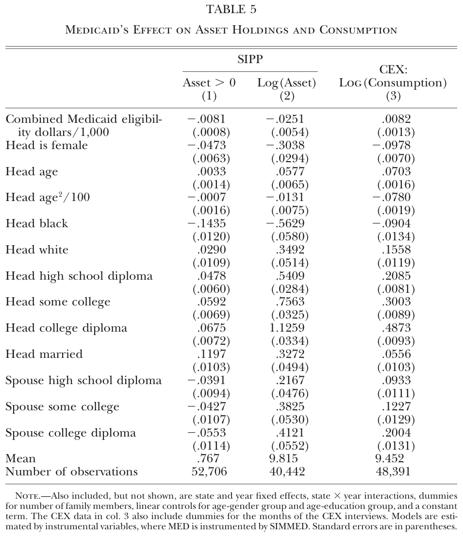
Our basic SIPP results are presented in columns | and 2 of table 5, where we show instrumental variables regressions that use as the dependent variable both a dummy for having any asset holdings and the log of asset holdings.19 We find a negative and highly significant effect of Medicaid in both specifications. For each $1,000 increase in Medicaid eligible dollars, there is a fall of 0.81 percent in the odds of having positive assets. Conditional on there being positive net wealth, we find that for each $1,000 of Medicaid eligible dollars, wealth holdings fall by 2.51 percent. These findings demonstrate that the Medicaid program has a sizable effect on savings behavior, which is consistent with a precautionary savings response to reduced risk of medical expenditure.
We can use these estimates to measure the net effect of the Medicaid program on asset holdings in 1993. Among those eligible for the Medicaid program, the average of Medicaid eligible dollars is $5,111.20 Thus, for this population, there is a reduction in the odds of having positive net worth of 4.2 percent and a reduction in net worth holdings of 12.8 percent. As an approximation, assume that those individuals who move from positive to zero net worth holdings would have otherwise had the median level of wealth among eligible positive wealth holders. This implies that the total reduction in net worth holdings due to Medicaid, if one accounts for individuals who reduce their wealth to zero, is 16.3 percent. Moreover, under the same assumption, we find that the expansions from 1984 to 1993 lowered wealth holdings among this population by 7.2 percent.
Table 5. MEDICAID’s EFFECT ON ASSET HOLDINGS AND CONSUMPTION
Notes: Nore.—Also included, but not shown, are state and year fixed effects, state X year interactions, dummies for number of family members, linear controls for age-gender group and age-education group, and a constant term. The CEX data in col. 3 also include dummies for the months of the CEX interviews. Models are estimated by instrumental variables, where MED is instrumented by SIMMED. Standard errors are in parentheses.
These are fairly sizable effects. While this effect is large for the relevant population, however, it is trivial relative to overall asset holdings in our sample because of the skewed nature of wealth holdings. The asset holdings of the eligible population in 1993 amounted to only 8.1 percent of the total asset holdings of our sample, despite the fact that this group is over 32 percent of our sample, because the mean net worth of eligibles is only one-quarter of the sample average. Thus the 16.3 percent reduction in net worth holdings for this group translates to only a 1.3 percent reduction in aggregate net worth holdings.
As discussed earlier, one potential concern with these results is sample selection since we are using only positive wealth observations in our log wealth models. If those moving from positive to zero savings were disproportionately high savers (above the mean for the sample), a negative effect on savings in the remaining sample would automatically be induced. But our small LPM coefficients make this unlikely. In particular, given that we find a reduction in the odds of being a positive saver of only 4.2 percent, we would require that those who move from being a positive saver to a nonpositive saver had wealth holdings, on average, of more than $44,000 for selection to explain our findings. It seems highly unlikely that Medicaid could be causing a reduction in wealth from more than $44,000 to zero, since for this population Medicaid eligible dollars average only $5,111.
The covariates have their expected effects. Wealth rises with age, is higher for whites and lower for blacks (relative to other nonwhites) and female heads, and rises with education and marital status. These effects are all highly significant.
These effects on the eligible population are very similar to the estimates of the previous literature on social insurance and savings. As noted above, Kantor and Fishback (1996) find that the introduction of workers’ compensation insurance lowered the savings of working households by 25 percent, and Engen and Gruber (1995) estimate that increasing the generosity of unemployment insurance by one-half would lower savings by 14 percent; both are similar to our 16.3 percent estimated effect of Medicaid on savings.
Dollar Effects
Evaluating our effects in dollar terms requires recognizing that the population that is affected by Medicaid is not representative of the full sample. In particular, given the skewed nature of wealth holdings, it is inappropriate to use the samplewide summary statistics from table 4. Moreover, summary statistics from our entire sample period incorporate the effects of the Medicaid expansions themselves, so that using them to evaluate our estimates would yield misleading results.
We therefore evaluate our estimates using only the 1984 sample, before Medicaid had expanded eligibility. For this sample, we compute actual eligibility for Medicaid, under both 1984 rules and 1993 rules, in the latter case inflating family income to 1993 levels. We then compute Medicaid eligible dollars for eligible families, under both 1984 and 1993 rules; eligible families are defined as families in which any member is eligible. Finally, we compute the weighted means of wealth only for the populations eligible in 1984 and 1993, where the weights are Medicaid eligible dollars. This weighted mean both is focused on the appropriate (eligible) population and places more weight on the families that are most affected by Medicaid policy.
Using this approach, we find that the Medicaid program lowers asset holdings by between 25 and 32 cents for each dollar of eligibility. The first of these figures uses just the log wealth coefficient, and the second incorporates the LPM effect as well, assuming that individuals who become nonpositive savers would have otherwise had the median positive level of savings. This implies that, among the eligible population, Medicaid lowered wealth holdings by between $1,293 and $1,645 in 1993 and that the expansions from 1984 to 1993 lowered wealth holdings by between $567 and $722.
Asset Tests
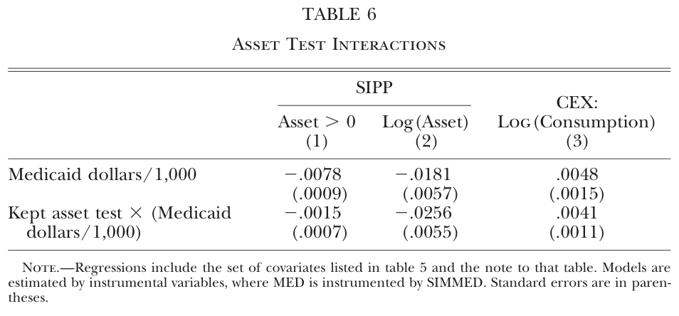
There is an ambiguous prediction for the interactive effect of asset testing with changes in Medicaid eligibility. Recall that over this period states were phasing out asset tests. We therefore explore the role of asset tests in table 6 by estimating models with a dummy for whether the state has an asset test, interacted with Medicaid dollars.
There is no dummy for the presence of an asset test per se since the asset test regime varies only by state and year, so that this is absorbed by our set of state X year dummies.
Notes: Nore.—Regressions include the set of covariates listed in table 5 and the note to that table. Models are estimated by instrumental variables, where MED is instrumented by SIMMED. Standard errors are in parentheses.
We find that there is in fact a negative interaction of eligibility with the presence of an asset test in columns | and 2, where wealth holdings are the dependent variable. For the regression for having positive assets, the interaction is marginally significant: it indicates that having an asset test raises the effect of a $1,000 increase in Medicaid eligible dollars from 0.78 percent to only 0.93 percent. For the log wealth regression, however, the interaction is highly significant and sizable; indeed, it is actually larger than the main effect on Medicaid eligible dollars. This indicates that for each $1,000 in Medicaid eligible dollars, there is only a 1.81 percent reduction in assets if there is no asset test in place, but there is a 4.37 percent reduction if there is an asset test in place. That is, having an asset test in place more than doubles the wealth reduction attributable to expanding Medicaid eligibility.
This pattern of effects should not be surprising: there should be much less effect of an asset test (at some positive level) on the odds of saving at all than on the amount of savings that are accumulated.
Thus our findings are consistent with the view that asset tests exacerbate the negative savings impact of the expansions by inducing wealth reductions in the population that is newly eligible on income grounds, but not on asset grounds.
Consumption Results
As noted earlier, Medicaid eligibility is predicted to have two positive effects on consumption: reduced precautionary savings and redistribution. We explore the effect of Medicaid eligibility on measured consumption expenditures by returning to column 3 of table 5. We show our basic specification, with the log of nondurable nonmedical expenditures as the dependent variable. As above, these regressions include not only the covariates shown in the table but also a full set of controls for ages of children /wives and full sets of dummies for states, years, and state X year interactions.
We find a highly significant positive effect of Medicaid eligibility on consumption, which is consistent with the negative effects on wealth holdings documented above. We estimate that for each $1,000 in eligibility, nondurable expenditures rise by 0.82 percent.
For the eligible population in 1993, this estimate implies that their consumption was 4.2 percent higher as a result of Medicaid eligibility. Once again, it is of interest to evaluate these effects in terms of dollars of increased consumption from the Medicaid expansions.
Following the same procedure as above, we find that in 1993, Medicaid raised the consumption of eligible families by $538. This effect is 33-42 percent as large as the effect on wealth holdings, which is consistent with the fact that the reduction in the stock of wealth is the cumulation of the flow effects of increased consumption. Comparing the precise magnitudes of the wealth and consumption effects is difficult and requires an underlying model of the accumulation process. Nevertheless, these findings confirm the basic results from the wealth data: Medicaid raises consumption and lowers savings.
We explore the role of asset tests in these data in column 3 of table 6. Once again, we use as our key regressors Medicaid dollars and an interaction of Medicaid dollars with a dummy for the presence of an asset test. And we once again find strong evidence with these consumption data for the proposition that Medicaid expansions reduce savings more when there is an asset test in place. The interaction coefficient is significant and roughly equal to the main effect on Medicaid dollars, indicating (as above) that the presence of an asset test doubles the consumption increase from expanded Medicaid eligibility. Taken together with the evidence for wealth holdings, our findings support the contention of Hubbard et al. (1995) that asset tests are an important determinant of savings (and consumption) behavior.
V. Conclusions
Theoretical advances in modeling precautionary savings over the past decade have raised the possibility that social insurance programs play an important role in determining both the level and distribution of asset holdings in the United States. Our results confirm that the parameters of the Medicaid program are a major determinant of the savings behavior of low-income households. We also confirm that households respond to asset testing on becoming eligible for Medicaid; eligibility has a much larger negative effect on savings if there is an asset test in place. On net, we find that in 1993 the Medicaid program lowered the wealth holdings of eligible households by 16.3 percent. We also find that the expansions of this program over the 1984—93 period lowered wealth holdings by 7.2 percent. Perhaps most important, we confirm that Medicaid lowers savings and raises consumption in two very different sources of data.
These findings therefore offer strong empirical support to the contention of Hubbard et al. (1995) that social insurance programs contribute to the skewed distribution of assets in the United States by lowering the savings of eligible low-income households.
At the same time, our findings offer some caution for the use of social insurance programs alone as an explanation for the level and distribution of U.S. wealth holdings. In aggregate, we estimate only a very small effect of Medicaid on asset holdings. Moreover, while our findings can explain some of the low asset holdings at the very bottom of the income distribution, there remains considerable skewness throughout the distribution (e.g., among those families above 200 percent of the poverty line) that cannot be explained by this or other means-tested programs. Of course, it is possible that means-tested social insurance can affect savings of higher-income households since these families may eventually become poor enough to qualify. Future work in this area could usefully explore how the sayings of noneligibles respond to changes in the generosity of means-tested social insurance.
The normative implications of our findings are somewhat unclear. On the one hand, precautionary saving for medical expenditures is a particularly inefficient means of insurance. When risks are large and variable, market insurance is a much more effective means of smoothing consumption than own savings. In this sense, our findings indicate increased efficiencies from expanded Medicaid eligibility that replaced self-insurance. On the other hand, there is substantial concern that savings are inefficiently low in the United States today. If there are other distortions in the economy that are causing our savings rate to be too low, then there could be large efficiency costs to reduced savings from social insurance programs. We view our findings as confirming the positive contention that means-tested social insurance programs are an important determinant of savings behavior. An important priority for future research is to understand the normative implications of these findings by exploring this trade-off between replacing inefficient self-insurance and lowering savings rates.
References
Abel, Andrew B. ‘‘Precautionary Saving and Accidental Bequests.’’ A.E.R. 75 (September 1985): 777–91.
Anderson, Patricia M., and Meyer, Bruce D. ‘‘The Incidence of a Firm-Varying Payroll Tax: The Case of Unemployment Insurance.’’ Working Paper no. 5201. Cambridge, Mass.: NBER, August 1995.
Browning, Martin, and Lusardi, Annamaria. ‘‘Household Saving: Micro Theories and Micro Facts.’’ J. Econ. Literature 34 (December 1996): 1797– 1855.
Carroll, Christopher D., and Samwick, Andrew A. ‘‘How Important Is Precautionary Saving?’’ Rev. Econ. and Statis. 80 (August 1998): 410– 19.
Currie, Janet. ‘‘Do Children of Immigrants Make Differential Use of Public Health Insurance?’’ Working Paper no. 5388. Cambridge, Mass.: NBER, December 1995.
Currie, Janet, and Gruber, Jonathan. ‘‘Health Insurance Eligibility, Utilization of Medical Care, and Child Health.’’ Q.J.E. 111 (May 1996): 431– 66. (a)
———. ‘‘Saving Babies: The Efficacy and Cost of Recent Changes in the Medicaid Eligibility of Pregnant Women.’’ J.P.E. 104 (December 1996): 1263–96. (b)
Curtin, Richard T.; Juster, F. Thomas; and Morgan, James N. ‘‘Survey Estimates of Wealth: An Assessment of Quality.’’ In The Measurement of Saving, Investment, and Wealth, edited by Robert E. Lipsey and Helen Stone Tice. Chicago: Univ. Chicago Press (for NBER), 1989.
Cutler, David M., and Gruber, Jonathan. ‘‘Does Public Insurance Crowd Out Private Insurance?’’ Q.J.E. 111 (May 1996): 391–430.
———. ‘‘Medicaid and Private Insurance: Evidence and Implications.’’ Health Affairs 16 ( January/February 1997): 194–200.
Dardanoni, Valentino. ‘‘Precautionary Savings under Income Uncertainty: A Cross-Sectional Analysis.’’ Appl. Econ. 23, no. 1, pt. B ( January 1991): 153–60.
Diamond, Peter A., and Hausman, Jerry A. ‘‘Individual Retirement and Savings Behavior.’’ J. Public Econ. 23 (February/March 1984): 81–114
Dubay, Lisa, and Kenney, Genevieve. ‘‘Did the Medicaid Expansions for Pregnant Women Crowd Out Private Coverage?’’ Health Affairs 16 ( January/February 1997): 185–93.
Dynan, Karen E. ‘‘How Prudent Are Consumers?’’ J.P.E. 101 (December 1993): 1104–13.
Employee Benefits Research Institute. ‘‘Sources of Health Insurance and Characteristics of the Uninsured.’’ Issue Brief no. 179. Washington: Employee Benefits Res. Inst., 1996.
Engen, Eric M., and Gruber, Jonathan. ‘‘Unemployment Insurance and Precautionary Saving.’’ Working Paper no. 5252. Cambridge, Mass.: NBER, September 1995.
Feldstein, Martin S. ‘‘Social Security, Induced Retirement, and Aggregate Capital Accumulation.’’ J.P.E. 82 (September/October 1974): 905–26.
———. ‘‘Social Security and Private Saving: Reply.’’ J.P.E. 90 ( June 1982): 630–42.
Fishback, Price V., and Kantor, Shawn Everett. ‘‘Did Workers Pay for the Passage of Workers’ Compensation Laws?’’ Q.J.E. 110 (August 1995): 713–42.
Fisher, Malcolm R. ‘‘Exploration in Savings Behaviour.’’ Bull. Oxford Univ. Inst. Statis. 18 (August 1956): 201–77.
Friedman, Milton. A Theory of the Consumption Function. Princeton, N.J.: Princeton Univ. Press (for NBER), 1957.
Gruber, Jonathan. ‘‘The Incidence of Mandated Maternity Benefits.’’ A.E.R. 84 ( June 1994): 622–41.
Gruber, Jonathan, and Krueger, Alan B. ‘‘The Incidence of Mandated Employer-Provided Insurance: Lessons from Workers’ Compensation Insurance.’’ In Tax Policy and the Economy, vol. 5, edited by David Bradford. Cambridge, Mass.: MIT Press (for NBER), 1991.
Guiso, Luigi; Jappelli, Tullio; and Terlizzese, Daniele. ‘‘Earnings Uncertainty and Precautionary Saving.’’ J. Monetary Econ. 30 (November 1992): 307–37.
Hansen, Gary D., and Imrohoroglu, Ayse. ‘‘The Role of Unemployment Insurance in an Economy with Liquidity Constraints and Moral Hazard.’’ J.P.E. 100 (February 1992): 118–42.
Hoynes, Hilary; Hurd, Michael; and Chand, Harish. ‘‘Imputed Wealth, Subjective Survival Probabilities, and Social Security Wealth.’’ Working paper. Cambridge, Mass.: NBER, 1995.
Hubbard, R. Glenn, and Judd, Kenneth L. ‘‘Social Security and Individual Welfare: Precautionary Saving, Borrowing Constraints, and the Payroll Tax.’’ A.E.R. 77 (September 1987): 630–46.
Hubbard, R. Glenn; Skinner, Jonathan; and Zeldes, Stephen P. ‘‘Precautionary Saving and Social Insurance.’’ J.P.E. 103 (April 1995): 360–99.
Intergovernmental Health Policy Project. Major Changes in State Medicaid and Indigent Care Programs. Edited by Debra J. Lipson, Rhona S. Fisher, and Constance Thomas. Washington: George Washington Univ., various editions.
Kantor, Shawn Everett, and Fishback, Price V. ‘‘Precautionary Saving, Insurance, and the Origins of Workers’ Compensation.’’ J.P.E. 104 (April 1996): 419–42.
Kennickell, Arthur B., and Starr-McCluer, Martha. ‘‘Changes in Family Finances from 1989 to 1992: Evidence from the Survey of Consumer Finances.’’ Fed. Reserve Bull. 80 (October 1994): 861–82.
Kotlikoff, Laurence J. ‘‘Health Expenditures and Precautionary Savings.’’ In What Determines Saving? by Laurence J. Kotlikoff. Cambridge, Mass.: MIT Press, 1989.
Kotlikoff, Laurence J.; Shoven, John; and Spivak, Avia. ‘‘Annuity Markets, Savings, and the Capital Stock.’’ In Issues in Pension Economics, edited by Zvi Bodie, John Shoven, and David A. Wise. Chicago: Univ. Chicago Press (for NBER), 1987.
Leimer, Dean R., and Lesnoy, Selig D. ‘‘Social Security and Private Saving: New Time-Series Evidence.’’ J.P.E. 90 ( June 1982): 606–29.
Powers, Elizabeth T. ‘‘Does Means-Testing Welfare Discourage Saving? Evidence from a Change in AFDC Policy in the United States.’’ J. Public Econ. 68 (April 1998): 33–53.
Rask, Kimberly, and Rask, Kevin. ‘‘Public Health Insurance and Moral Hazard.’’ Manuscript. Hamilton, N.Y.: Colgate Univ., 1995.
Sheiner, Louise. ‘‘Health Care Costs, Wages, and Aging: Assessing the Impact of Community Rating.’’ Manuscript. Washington: Fed. Reserve Bd., 1996.
Sheshinski, Eytan, and Weiss, Yoram. ‘‘Uncertainty and Optimal Social Security Systems.’’ Q.J.E. 96 (May 1981): 189–206.
U.S. House of Representatives. Committee on Ways and Means. Background Material and Data on Programs within the Jurisdiction of the Committee on Ways and Means. Washington: Government Printing Office, 1994.
Yelowitz, Aaron S. ‘‘The Medicaid Notch, Labor Supply, and Welfare Participation: Evidence from Eligibility Expansions.’’ Q.J.E. 110 (November 1995): 909–39.
Printed notes
1. From authors’ tabulations of the Survey of Income and Program Participation data described below; assets are total household net worth.
2. A number of states have even expanded coverage above 185 percent of poverty for pregnant women and infants, using only state funds with no federal match.
3. There were additional expansions for older groups of children as well, but this table usefully illustrates the variation in eligibility that we exploit in our estimation.
4. For a dissent using a very different methodology, see Dubay and Kenney (1997); see also the response in Cutler and Gruber (1997).
5. In fact, over the entire lifetime, the consumption effect is ambiguous. When there is no bequest motive, individuals will eventually desire to run down their stock of precautionary savings against medical risk as they near the end of life and the total stock of future risk shrinks. Thus reduced income risk will raise consumption today but may lower it close to the end of life. In our empirical work, however, we focus on families with no members over age 64, so that for this younger sample there should be only negative effects of medical risk on consumption and thus positive effects of increases in Medicaid eligibility.
6. Modeling the precautionary motive for wealth accumulation has a long tradition, dating at least back to Fisher (1956) and Friedman (1957); see Deaton (1992) and Browning and Lusardi (1996) for reviews of recent developments. A natural implication of precautionary saving models is that social insurance programs, by reducing income or expenditure risk, will reduce asset accumulation. This point has been made in the context of the Social Security program by Sheshinski and Weiss (1981), Abel (1985), Hubbard and Judd (1987), and Kotlikoff, Shoven, and Spivak (1987) and in the context of the unemployment insurance program by Hansen and Imrohoroglu (1992) and Engen and Gruber (1995). A more general treatment of social insurance and precautionary savings was introduced by Hubbard et al. (1995), who consider the distributional impacts of social insurance as well as its effect on average savings and incorporate the role of asset testing.
7. These insurance payments may have been explicit, through the purchase of individual insurance or employer premium-sharing arrangements, or implicit, through reduced wages for those provided insurance by their employers. Evidence for such implicit payments is presented in Gruber and Krueger (1991), Gruber (1994), and Sheiner (1996).
8. The value of a family’s home is excluded from this asset test for AFDC, and the value of an automobile (up to $1,500) is excluded as well (U.S. House of Representatives 1994). The Medicaid expansions allowed families in states retaining asset tests to have asset holdings that were less than the supplemental security income asset limit of $2,000 rather than the AFDC asset limit of $1,000.
9. For the case of workers’ compensation, see Gruber and Krueger (1991) and Fishback and Kantor (1995); for the case of unemployment insurance, see Anderson and Meyer (1995).
10. In Kantor and Fishback’s (1996) sample, only 10 percent of individuals hold accident insurance. There is very little private unemployment insurance in the United States. Annuitization against mortality risk is very uncommon at the individual level, although many individuals are partially annuitized through firm pension plans.
11. The first wealth supplement for 1985 was actually in the third interview. There was no survey in 1989, and the 1988 survey did not contain a complete wealth inventory.
12. This includes semidurables such as clothing; it excludes spending on housing and housing durables. We do not include these items because they may be a form of savings rather than consumption.
13. Making a dollar eligible for Medicaid is not the same as actually providing a dollar of insurance coverage, since in practice a large share of our sample will not take up the coverage for which they are eligible; see Currie and Gruber (1996a, 1996b) and Cutler and Gruber (1996) for a further discussion. For the purposes of our analysis, however, Medicaid eligibility is the more relevant concept. As emphasized by Hubbard et al. (1995), it is the option of taking up social insurance that affects savings behavior, even among those who are not in the program at a point in time. By the same token, of course, it may be that even those ineligible for the program respond to the inherent savings disincentives since they may become eligible. To the extent that such a response exists, our estimates, which focus just on the eligible population, will understate the savings effect of the Medicaid program.
14. This normalization has two potential weaknesses. First, it is possible that the value of Medicaid is not determined by area-specific costs; it may be that the value is viewed in terms of services provided, not in terms of the costs of those services. But it seems more likely that individuals do consider the cost of services since Medicaid is contrasted with either no insurance or private insurance, both of which will be more costly as medical costs are higher. Second, this measure captures not only price variation but also variation in utilization of services by the Medicaid population. But utilization variation may also capture the quality of the Medicaid program, e.g., by representing the ease with which Medicaid patients can see providers in those states. In any case, our results are very similar if we do not use this deflator and instead simply use national average expenditures to form our measure.
15. We use the CPS, and not the SIPP or CEX, for this step of the analysis since the larger sample sizes guarantee a sufficient sample in each cell. Since we are simply imputing averages by cell, we can easily estimate the averages in the CPS and then carry them over to these other data sets. This also has the virtue that we use the same Medicaid eligibility construct in both the CEX and the SIPP.
16. To illustrate, suppose that high school dropouts in Alabama have particularly low incomes (and therefore low savings), relative to high school dropouts elsewhere and relative to other education groups in Alabama. If we used the actual sample of high school dropouts in Alabama, we would assign them a high fraction eligible on the basis of their low incomes. We would then find a spurious negative association between eligibility and savings since they also have low savings. By using a nationally representative sample, we avoid this problem since we are using only the laws of Alabama, and not the characteristics of its residents, to impute eligibility. It is worth noting that we carry out this exercise quarterly, to account for within-year variation in the timing of the expansions, and that we then match to the precise quarterly timing of the SIPP and CEX.
17. Wealth and consumption are measured in real 1987 dollars to match the timing of the NMES medical spending information used to create MEDj.
18. They include four dummies for the education of the head and separate dummies for each of the age/education categories of women who might be eligible for pregnancy coverage.
19. We have estimated the reduced-form version of this model using both this linear probability model (LPM) specification and a probit specification. The results are identical, so we use the LPM specification here for ease of instrumental variables estimation.
20. This number is much larger than the figure in table 3 for 1993 since it is conditional on Medicaid eligibility.