Adverse selection in the group life insurance market

Timothy F. Harris; Aaron Yelowitz; Jeffery Talbert; Alison Davis

Economic Inquiry, published early-view edition (2023), pages 1–31. https://doi.org/10.1111/ecin.13159

Received: 13 April 2022. Accepted: 12 May 2023. © 2023 Western Economic Association International.

Author affiliations: Department of Economics, Illinois State University, Normal, Illinois, USA (Harris); Department of Economics, University of Kentucky, Gatton College of Business and Economics, Lexington, Kentucky, USA (Yelowitz); Department of Pharmacy Practice and Science, University of Kentucky, Lexington, Kentucky, USA (Talbert); Department of Agricultural Economics, University of Kentucky, Lexington, Kentucky, USA (Davis).

Correspondence: Aaron Yelowitz, aaron@uky.edu.

Funding information: National Institutes of Health, Grant/Award Number UL1TR001998. Managing Editor: Farasat Bokhari.

Abstract

The employer‐sponsored life insurance (ESLI) market is susceptible to adverse selection due to community‐rated premiums, guaranteed issue coverage, and the existence of an individual market. Using payroll and healthcare claims data from a large university, we find that employees with worse health are more likely to elect coverage causing adverse selection in supplemental ESLI. Nonetheless, we find employees typically do not increase coverage following a severe illness even when they can without providing evidence of insurability. Furthermore, demand estimation shows employees are not price‐sensitive and estimated increases in premiums from adverse selection are unlikely to cause significant welfare loss.

Keywords: adverse selection, employer‐sponsored insurance, life insurance
JEL classification: D82, G22, J33

Abbreviations: ACLI, American Council of Life Insurers; ACS, American Community Survey; ATT, average treatment on the treated; BLS, Bureau of Labor Statistics; CCI, Charlson Comorbidity Index; CDC, Centers for Disease Control and Prevention; COPD, Chronic Obstructive Pulmonary Disease; EOI, evidence of insurability; ER, emergency room; ESHI, employer‐sponsored health insurance; ESLI, employer‐sponsored life insurance; FDR, false discovery rate; HRS, health and retirement study; LTD, long‐term disability; NCS, National Compensation Survey; SIPP, Survey of Income and Program Participation.

1. INTRODUCTION

Life insurance is one of the largest private insurance markets in the United States. In 2021, life insurance coverage totaled $20.4 trillion (ACLI, 2021), and individuals paid $145.1 billion in life insurance premiums in 2019 (Federal Insurance Office, 2020).¹ Notwithstanding widespread coverage, large disparities still exist between life insurance holdings and underlying vulnerabilities, with some estimates exceeding $15 trillion (Bernheim et al., 2003; Conning, 2014; LIMRA, 2015b). Adverse selection in life insurance—where higher‐risk individuals are more likely to purchase coverage leading to market failure—could be one of the causes of these uninsured vulnerabilities.

We use detailed administrative data from a large public university (“the University” henceforth) to test for adverse selection in employer‐sponsored life insurance (ESLI). Supplemental ESLI at the University is particularly susceptible to adverse selection for several reasons. First, supplemental ESLI is “guaranteed issue” (cannot deny coverage based on health) and priced based on the group's risk rather than individual health characteristics. Second, employees at the University may increase supplemental ESLI coverage annually without individual underwriting (health screening) in many instances. As a result, individuals who receive negative health information (e.g., cancer diagnosis) may increase coverage prior to death and receive significantly higher payouts. Third, there are substantial differences in the levels of coverage available at the University, which allows for adverse selection on not only the extensive margin (participation in supplemental ESLI) but also on the intensive margin (level of supplemental coverage). Fourth, individual term life insurance represents a viable alternative to ESLI. In contrast to the ESLI, term life insurance is individually underwritten (experience‐rated) and is not guaranteed issue. Consequently, term life insurance offers significantly cheaper premiums than ESLI for healthy University employees, potentially drawing the good risks away from the ESLI pool.

Overall, these factors provide ample opportunity for adverse selection in ESLI at the University and could theoretically lead to a “death spiral” or complete unraveling of the ESLI market. However, supplemental ESLI with similarly structured policies is widespread despite these factors, indicating a lack of the most severe adverse selection. Nonetheless, even in the absence of complete market breakdown, adverse selection can still lead to elevated premiums, welfare loss, and underinsurance.

Notwithstanding the potential for adverse selection, several factors might temper it in this market. For instance, inertia in employee elections is well‐documented and can lead to decreased levels of adverse selection (Handel, 2013).

Furthermore, heterogeneity in preferences (i.e., multiple dimensions of selection) can cause increased participation by those with lower mortality risk, thus attenuating adverse selection (Cutler et al., 2008; Finkelstein & McGarry, 2006).

Consequently, the existence and magnitude of adverse selection in ESLI is an empirical question. Using the widely implemented positive correlation test, we find robust evidence of adverse selection in supplemental ESLI at the University. The analysis shows that employees with severe health ailments, as indicated by diagnostic codes in the administrative data, are more likely to have supplemental ESLI coverage. Nonetheless, we do not find evidence that individuals increase coverage levels following a significant negative diagnosis, consistent with inertia or inattention. To gauge the magnitude of the adverse selection, we use a metric for individual probability of death based on the Charlson Comorbidity Index (CCI) to derive expected costs of elected coverage. We then compare the expected costs of the adversely selected sample of employees to random draws of employees at the University. We find that expected costs are in the 97.0% or 9.7% more than the median expected cost of the random draws.

The magnitude of these elevated costs on welfare is contingent on the price elasticity of demand, which we estimate using the discontinuous pricing structure of the University's ESLI policy. We find that employees have very inelastic demand for supplemental coverage, which implies that market distortions and welfare loss from the adverse selection are likely minimal. Furthermore, we note that supplemental ESLI coverage is conditional on employment and that workers that separate from their employer—including those who leave due to deteriorating health—typically lose ESLI coverage. The conditional nature of insurance weakens the relationship between mortality risk, actual payouts, and premiums. In short, adversely selected coverage only impacts pricing inasmuch as the employees pass away while employed.

This paper contributes to the significant literature on adverse selection in insurance markets. Adverse selection has been analyzed in health insurance (Cardon & Hendel, 2001; Cutler, 2002; Cutler & Reber, 1998; Einav et al., 2010; Sasso & Lurie, 2009; Simon, 2005), long‐term care insurance (Finkelstein & McGarry, 2006; Oster et al., 2010), and annuities (Finkelstein & Poterba, 2004). This literature illustrates the heterogeneous influence of adverse selection on markets and the importance of contractual arrangements in insurance plans. With regard to life insurance, previous empirical work on adverse selection primarily focuses on the individual market. The seminal paper by Cawley and Philipson (1999) finds no evidence of adverse selection in the term life insurance market. Subsequent work has mixed results (Harris & Yelowitz, 2014; He, 2009, 2011; Hedengren & Stratmann, 2016).

These studies provide valuable insights into one portion of the life insurance market, but little attention has been given to the ESLI market, which constitutes 37% of total life insurance coverage in 2020 (ACLI, 2021). Hedengren and Stratmann (2016) is the only empirical study, to our knowledge, that analyzes adverse selection in the ESLI market.

Their study finds “weak evidence” of adverse selection in ESLI using data from the Survey of Income and Program Participation (SIPP) linked with administrative records. While their study contributes to the literature, the analysis of ESLI is limited by their data. Specifically, the SIPP panels do not contain information on ESLI availability, provision by employers, or differentiate between basic and supplemental life insurance coverage.

This study advances the literature by using administrative healthcare and payroll data at the individual level to analyze adverse selection in supplemental ESLI. The detailed data and our comprehensive understanding of policies allow us to test the individual and institutional components that, in theory, should lead to adverse selection. This research also contributes to the literature on the interaction between community‐rated premiums and adverse selection (Buchmueller & Dinardo, 2002). Lastly, this paper advances the knowledge of individual responses to receipt of negative health information.

2. LIFE INSURANCE OVERVIEW

In 2020, 105 million employees were covered by ESLI, with coverage totaling $7.5 trillion (ACLI, 2021). ESLI customarily has an automatic portion provided by the employer (basic coverage) and an option to purchase additional coverage through payroll deductions with after‐tax dollars (supplemental coverage). Three‐quarters of all full‐time workers had access to ESLI (U.S. Department of Labor, 2015), and about half of all workers had access to supplemental ESLI coverage (LIMRA, 2015a). Based on SIPP data, 51% of employed adults have life insurance coverage. Of employed individuals with life insurance coverage, 58% have some ESLI coverage, and 34% exclusively have ESLI coverage. The statistics for university employees are similar, with 55% having life insurance and, conditional on having some coverage, 63% have ESLI, and 36% exclusively have ESLI.² As mentioned, ESLI is generally community‐rated, meaning that premiums are a function of the expected costs of the insured group rather than a single individual's probability of death. More explicitly, ESLI premiums generally only adjust based on age and do not use additional individualized information on health or other risk factors.

The individual market accounts for 63% of life insurance coverage (ACLI, 2021). Within the individual market, policies are differentiated by term and whole life insurance.³ Term life insurance provides coverage for a specified period (typically ranging from 10 to 30 years) and pays the policy's face value upon the death of the policyholder. Term life insurance accounts for 74% of the face value of individual life insurance policies (ACLI, 2021) and is a close substitute for supplemental ESLI.

In contrast to ESLI, term life insurance is experience rated, meaning that premiums vary based on individual characteristics, including age, gender, smoking status, health status, family history, and participation in risky behaviors.

This underwriting represents a cost to applicants as it commonly requires a medical examination, blood work, and detailed medical history. The most common form of term life insurance is a level term policy, which keeps premiums constant over the life of the policy.

3. EXPECTED ADVERSE SELECTION IN ESLI

As discussed in the introduction, several aspects of ESLI could lead to adverse selection. This section provides further motivation about adverse selection in the ESLI market.

3.1. Differences in probability of death: Community-rated/guaranteed issue

Guaranteed issue coverage and community‐rated premiums that only adjust based on age could cause adverse selection in ESLI at the University.⁴

These features imply that employees in the same age bin of varying health can purchase policies for equal premiums.⁵ For example, employees aged 45 through 49 all pay the same premium per $1000 in coverage. However, within that age bin, the probability of death for those in the fifth percentile is 63 per 100,000 while those in the 95th percentile is 1856 per 100,000.⁶

Thus, combining guaranteed issue with community‐rated premiums provides significant opportunities for adverse selection.

3.2. Ability to increase coverage following diagnosis

Another feature of the University's ESLI policy that could exacerbate adverse selection is the ability to ratchet up coverage without medical underwriting. A significant portion of University employees can increase coverage by 1× salary each year without proof of insurability, which means that on average, they can increase coverage within 6 months of a diagnosis with the elected higher coverage going into effect shortly thereafter. Consequently, individuals that receive negative health information or are diagnosed with a life‐threatening condition may increase coverage. A simple example helps illustrate how only a few employees with anticipated deaths can cause significant adverse selection. Suppose that a typical employer plan that covers 15,000 employees has 50 deaths per year and that half of all employees who die have supplemental coverage and equal salaries. Further suppose that the average employee receives a payout of 1× salary. Given these assumptions, only six employees who pass away would have to increase coverage to the maximum of 5× salary to cause payouts to double.

However, employees will only ratchet up coverage inasmuch as they are aware of pending death. Data on 1367 deaths, as reported in the Health and Retirement Study (HRS), shed light on the degree of anticipation of death.⁷

Follow‐up exit interviews of surviving relatives show that 44.7% of deaths were expected and that roughly a quarter of all deaths resulted from an illness diagnosed at least a year prior to the individual's death.⁸⁹

3.3. Differences in benefit levels

Another critical aspect of ESLI that could increase adverse selection is the wide range of coverage offered. Employees at the University may ultimately elect supplemental coverage from 1× salary to 5× salary without medical underwriting inasmuch as the policy does not exceed the guaranteed issue amount ($375,000). Cutler and Reber (1998) illustrate how adverse selection in the presence of different levels of generosity can significantly affect health insurance markets. They document an insurance “death spiral” where adverse selection led to the discontinuation of the most generous health insurance plan at Harvard University after the university stopped subsidizing the policy. They noted that this problem is not an isolated occurrence, and many such employer‐sponsored health insurance (ESHI) plans cannot offer policies with significant differences in generosity (unless the employer differentially subsides the more generous option).¹⁰

In contrast to ESHI plans, supplemental ESLI plans where the highest coverage can be 5× more generous than the lowest coverage option are common. Furthermore, supplemental ESLI commonly lists a single price per $1000 in coverage regardless of the amount purchased. Consequently, intensive margin adverse selection would increase premiums for all employees at a specific employer, and not only for those that elect the most generous coverage. Overall, there is room for high‐risk individuals to not only exhibit adverse selection on the extensive margin of supplemental coverage, but also on the intensive margin.

3.4. Viable outside option: Non-group life insurance

The last major factor that influences adverse selection in the ESLI market is the existence of a functioning, competitive term market. In stark contrast to ESLI, term policies are individually underwritten based on the policy's term length and face value (amount payable at death). Consequently, healthy employees may generally purchase term life insurance for lower rates than supplemental ESLI.

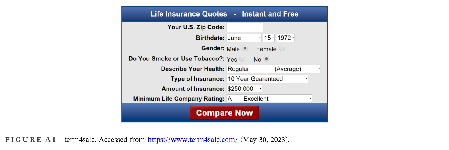
To understand the difference in premiums between ESLI and term coverage, we use scraped premiums from term4sale.com (N = 5.85 million quotes). Term4sale is a life insurance quoting website run by CompuLife that provides life insurance quoting software to insurance agents.¹¹

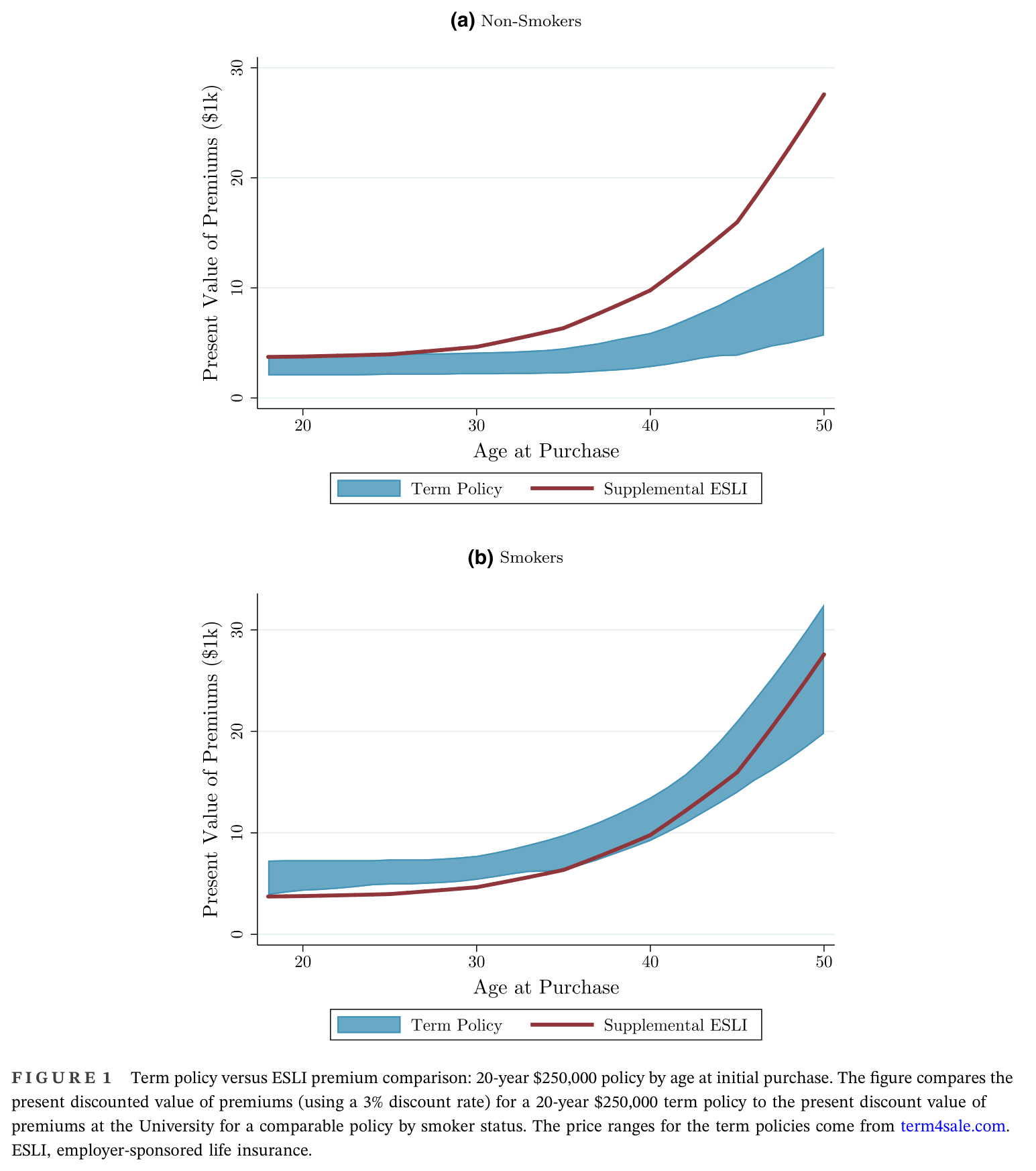
The website uses age, gender, health status, and smoking status to quote relevant insurance products currently on the market.¹² Figure 1 compares the range of prices (present value of premiums) for a 20‐year $250,000 policy in the term life insurance market to the present value of premiums for a comparable policy for 20 years at the University. As shown in Figure 1a, premiums for supplemental ESLI generally exceed the range of premiums for term life insurance for non‐smokers. For example, a 40‐year‐old, non‐smoking female employee without any health problems (Preferred Plus category) will save $6988 ($349 annually) by purchasing a $250,000 term life insurance policy in the non‐group market rather than electing the same amount in supplemental ESLI through the university. However, as shown in Figure 1b, smokers can get cheaper coverage through the University relative to a term life insurance policy due to the community‐rated premiums at the University. Consequently, these differences could lead to significant levels of adverse selection in supplemental ESLI.

In addition to cheaper coverage, another advantage of term life insurance is that the policy is only contingent on premium payments. In contrast, ESLI coverage is conditional on employment at the given institution. If an individual has ESLI coverage but switches jobs, he or she will generally not be able to continue the same coverage.¹³

If the new employment does not offer ESLI, the individual will need to turn to the term market for coverage. If an individual purchases term coverage later in life (due to lapsing ESLI coverage), he or she is more likely to have medical conditions that trigger higher rates. Therefore, the conditional nature of ESLI should also influence employees to purchase term coverage rather than ESLI.

Even though there are significant potential savings depending on the employee's age, the term of the policy, and the face value, there are also higher fixed costs associated with term life insurance relative to supplemental ESLI. Supplemental ESLI has the advantage of payroll deductions, a simplified choice set, and generally no medical underwriting.

In addition, since employees elect supplemental ESLI in multiples of income, coverage automatically adjusts for changes in salary. The implicit costs of determining the best policy from a wide array of options, and the inconvenience of medical exams and intrusive questions, might induce individuals to purchase the simplified ESLI policy. Nonetheless, the significant savings from the term market have the potential to overcome these costs.

Overall, the setup of ESLI and the existence of the term market allow for significant adverse selection in the ESLI market.¹⁴

Figure 1. Term policy versus ESLI premium comparison: 20‐year $250,000 policy by age at initial purchase

Term policy versus ESLI premium comparison: 20‐year $250,000 policy by age at initial purchase. The figure compares the.

3.5. Offsetting effects

Despite the factors outlined above, there are countervailing influences that might mitigate adverse selection or potentially cause advantageous selection where individuals of higher risk are less likely to purchase coverage.

Several studies have illustrated that the standard one‐dimensional model of asymmetric information (i.e., health and insurance elections) is insufficient when characterizing asymmetric information (Cutler et al., 2008; De Meza & Webb, 2001). For example, Finkelstein and McGarry (2006) find that the prevalence of healthy risk‐averse individuals who purchase coverage offset the adverse selection, which leads to a lack of a positive correlation between risk and coverage. Similarly, Fang et al. (2008) find that individuals with higher cognitive abilities are lower risk and are more likely to purchase Medigap policies, thus resulting in advantageous selection. These studies, among others, illustrate that preference‐based selection can potentially counteract or, in some instances, exacerbate adverse selection. In the case of ESLI, if employees have strong tastes for life insurance and are low risk, then the overall correlation between risk and coverage might even be negative, implying advantageous selection.

Another potential factor that could decrease adverse selection in the ESLI market is inertia. Handel (2013) show in the context of ESHI that inertia significantly reduced the amount of adverse selection and that welfare loss doubles in its absence. In the case of supplemental ESLI, many employees make an initial election and then forget about it as it represents a small budget share. If employees were forced to make an active choice regarding supplemental ESLI elections every year, then adverse selection would likely increase as it did in ESHI. Nonetheless, diagnosis with a significant illness provides significant incentives to understand the available options and respond accordingly.

4. UNIVERSITY LIFE INSURANCE

Qualified employees at the University are automatically provided basic life insurance coverage of 1× annual salary.¹⁵¹⁶ In addition to this coverage, employees may elect supplemental life insurance in multiples of their annual salary through payroll deductions on an after‐tax basis. These elections must occur during annual open enrollment periods or after a qualifying event, including birth, adoption, marriage, divorce, or employment status change.¹⁷

Depending on the timing and amount of supplemental life insurance elections, employees may be subject to individual underwriting and required to provide “evidence of insurability” (EOI). Providing EOI entails filling out a medical history form and, in some cases, a medical examination to verify the employee is “insurable.” Elections by new hires do not require EOI if the coverage level does not exceed either 3× annual salary or the guaranteed issue amount of $375,000.¹⁸

Furthermore, employees may increase coverage by 1× salary each year during open enrollment without EOI inasmuch as the total face value does not exceed the guaranteed issue amount or 5× annual salary. This means that within 2 years of being hired, employees that earn up to $75,000 can have 5× annual salary in supplemental ESLI without providing any personal health information to the insurance company. Outside of new hire elections and annual increases by those who already had supplemental coverage, all other supplemental ESLI elections require EOI, wherein the insurance company may reject requests to increase or start coverage. Overall, employees may provide EOI and elect up to the lesser of 5× annual salary or $1,000,000 during an open enrollment period.¹⁹²⁰ As is typical with ESLI, premiums at the University are community‐rated and do not account for differences in health. The premiums are differentiated solely by 5‐year age bins.

4.1. Representativeness

Given that we analyze a single university, it is important to understand how representative the University is of other universities and firms to gauge the external validity of the findings. Using the National Compensation Survey (NCS) conducted by the Bureau of Labor Statistics (BLS), Harris and Yelowitz (2017) show that the basic ESLI coverage for the University is within the norm for other colleges and universities. However, the NCS does not have information about supplemental ESLI coverage. To get a sense of standard features in supplemental ESLI policies, this study analyzes benefit books collected from more than 400 universities. Of all the universities surveyed, 70 universities had well‐ documented information on both basic and supplemental coverage. The average guaranteed issue amount (amount available without proof of insurability) for those universities is $254,344 with a maximum guaranteed issue amount of $750,000.²¹

The University's guaranteed issue amount of $375,000 is not out of the ordinary in comparison to the other universities and colleges sampled. From the survey of benefit books, all but one University adjust supplemental premiums based solely on age. Roughly half of the plans with requisite details allow employees to increase coverage without proof of insurability during open enrollment periods. The approved increases range from $5000 to $300,000 with the mode of 1× annual salary. It is less common for employees to be able to elect coverage without evidence of insurability if they did not elect supplemental ESLI when they were initially hired. Overall, it appears that the ESLI at the University in this study fits within the norm for colleges and universities regarding guaranteed issue amounts and underwriting but is on the more generous side of allowing employees to enroll/increase coverage during open enrollments. Consequently, if there is no evidence of significant adverse selection at the University with a vulnerable ESLI structure, there is likely no significant adverse selection at less generous institutions.

5. DATA

We use administrative payroll data from the University in a panel from 2013 to 2018 as the primary data source. These data include information on benefit elections (e.g., health insurance, retirement contributions, life insurance), annual salary, employment information (e.g., hire date, faculty/staff), and demographics. The main analysis sample we use consists of 19,484 unique active full‐time university employees who participate in ESHI (i.e., those with healthcare data).²²²³ We use University healthcare claims data to derive measures of individual mortality risk, which are required to analyze the existence of adverse selection. These data include Clinical Classifications Software codes, rounded healthcare expenditures, and the number of hospital stays for each employee in our sample. To quantify mortality risk, we focus on 17 major clinical conditions included in the CCI (Charlson et al., 1987).²⁴

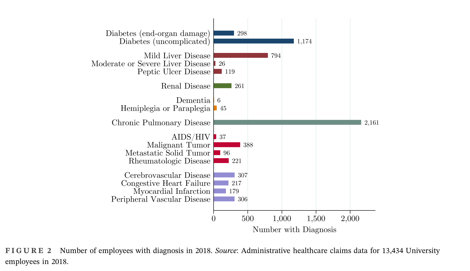
The CCI was developed specifically to analyze mortality risk in longitudinal studies and is widely used in academic research (e.g., Chandra et al., 2014; Chaudhry et al., 2005; Sundararajan et al., 2004). Figure 2 presents the number of diagnoses for each of the CCI clinical conditions for full‐time University Employees in 2018. The most common diagnoses include Chronic Pulmonary Disease (2161), Diabetes (uncomplicated) (1174), Mild Liver Disease (794), and malignant tumor (388). The least common diagnoses for University employees are Dementia, Moderate/Severe Liver Disease, AIDS/HIV, and Hemiplegia/Paraplegia, with each affecting less than 50 employees.²⁵ Conditional on having a CCI diagnosis, 33.0% have more than one in 2018.

Figure 2. Number of employees with diagnosis in 2018

Number of employees with diagnosis in 2018. Source: Administrative healthcare claims data for 13,434 University.

An advantage of using CCI for a measure of health is that the scores are designed to produce an individual's expected probability of death.²⁶ To construct a probability of death metric for the sample, we follow Charlson et al. (1987) to calculate a 1‐year probability of death for University employees with at least one of the diagnoses.²⁷

The traditional use of the CCI would assign everyone without one of the 17 diagnoses the same probability of death. Nonetheless, there is heterogeneity in mortality risk by age, race, gender, education, and marital status for those without a CCI diagnosis.²⁸

To leverage this heterogeneity, we use data from the Centers for Disease Control and Prevention (CDC) National Vital Statistics System Mortality Multiple Cause‐of‐Death Files from 2008 to 2017. These data include the universe of deaths in the United States with information on race/ethnicity, gender, marital status, and education.²⁹

We aggregate the total number of deaths for each unique group and use this metric as the numerator in our probability of death metric. We use the weighted count of each socioeconomic group derived from the American Community Survey (ACS) from the same years for the denominator. The probability of death metric for those without one of the 17 diagnoses is simply the proportion of deaths per the population of each subgroup. For example, there is an average of 3738 deaths per year for individuals that are age 50, male, not married, white, and have a staff‐level education. On average, there are 403,337 individuals in the U.S. for this sociodemographic group across the sample years. Therefore, for this group, the 1‐year mortality rate is 927 in 100,000. We make a final adjustment to this metric by increasing the probability of death for individuals in the sample that use tobacco as reported in the claims data.³⁰

Although using this metric of the probability of death for those without a CCI diagnosis should increase the accuracy relative to the assignment of a single probability of death for the entire group, there are still a couple of non‐ trivial limitations. First, the universe of fatalities in the U.S. contains individuals with one or more of the 17 CCI diagnoses. Consequently, the calculated probabilities of death for each subgroup likely exceed the actual risk for the group without one of the 17 diagnoses. Second, employed individuals have a significantly lower mortality risk than unemployed individuals (Roelfs et al., 2011). Thus, the population of University employees is likely at a lower risk than the entire population, causing this metric to again overstate risk. Nonetheless, the constructed probability of death metric for those without one of the CCI diagnoses should be highly correlated with actual risk and valuable for analyzing adverse selection.

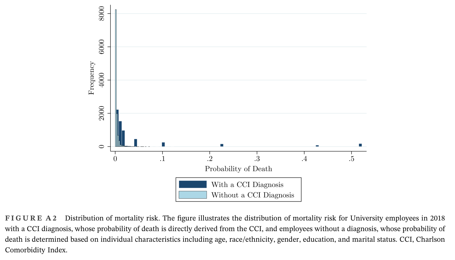
We combine the CCI probability of death for those with one of the diagnoses with the probability of death metric derived using CDC and ACS data. The vast majority of the risk and variation comes from those with at least one of the 17 diagnoses (mean 4.5% and s.d. 11.0% for 1‐year mortality risk), whereas the risk and variation for those without one of the diagnoses is significantly smaller (mean 0.3% and s.d. 0.4³¹%).

The combined metric arguably capture a significant amount of the heterogeneity in mortality risk for university employees. Nonetheless, in the main analysis, we report both the CCI results and the constructed probability of death estimates to mitigate concerns that measurement error is driving our main findings.

While the probability of death metric arguably captures mortality risk well in general, given the conditional nature of ESLI, ideally we would use a measure of mortality risk while employed. Nonetheless, it is likely that the probability of death while employed is highly correlated with the general probability of death, but that the risk, conditional on employment is lower. One factor supporting this correlation is that University employees who qualify for long‐term disability (LTD) may continue ESLI coverage even when physical limitations disallow full‐time employment.

Notwithstanding, it would be optimal to have data that contains mortality information and employment status for the general population to gauge the difference between the conditional and unconditional probabilities of death. We are unaware of such data and even if these data were available, it is even less likely that they would contain detailed information on an individual's health (e.g., CCI). Consequently, we would only be able to impute this probability of death metric based on broad demographic characteristics (e.g., age, race, gender) with additional data.

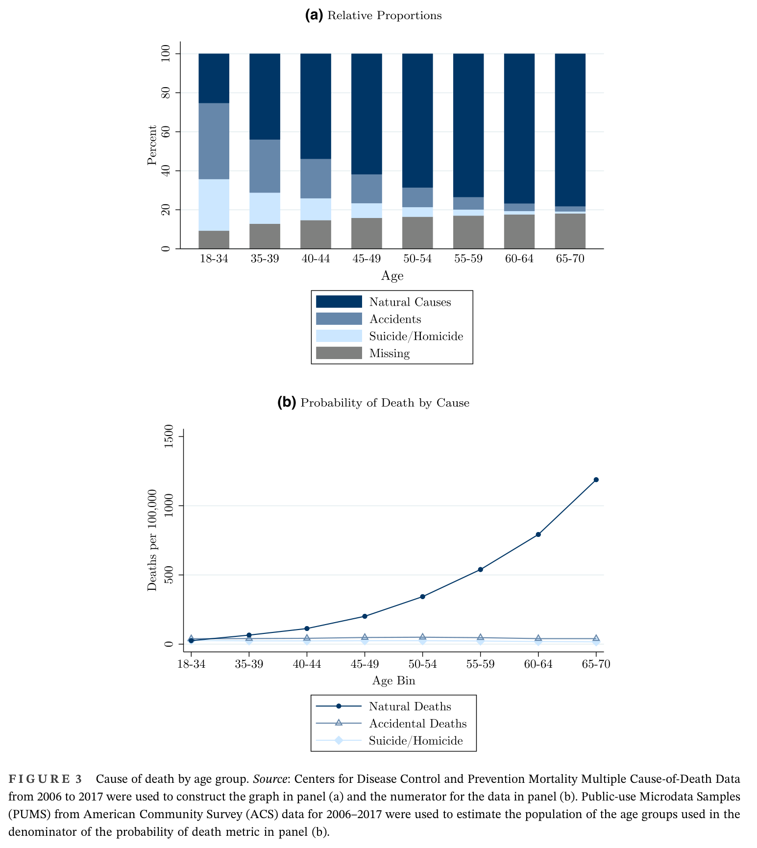
While we do not have these data, companies that offer ESLI have extensive data on risk and expected costs for employed individuals and price their policies accordingly. ESLI premiums increase significantly with age reflecting higher payouts for older employees. If every employee who passed away due to an illness exited the University and lost coverage before death, then the ESLI premiums should primarily reflect the risk of accidental death. As illustrated in Figure 3, the proportion of accident‐related deaths decreases with age and the probability of accidental death is relatively flat across ages. Thus, the increasing premiums with age better reflect deaths due to “natural” (i.e., health‐related) causes, which is arguably captured by our probability of death metric derived from diagnostic codes. In short, we acknowledge the limitations of our risk metric, but we argue that it still meaningfully captures the relevant risk for ESLI.

5.1. Summary statistics

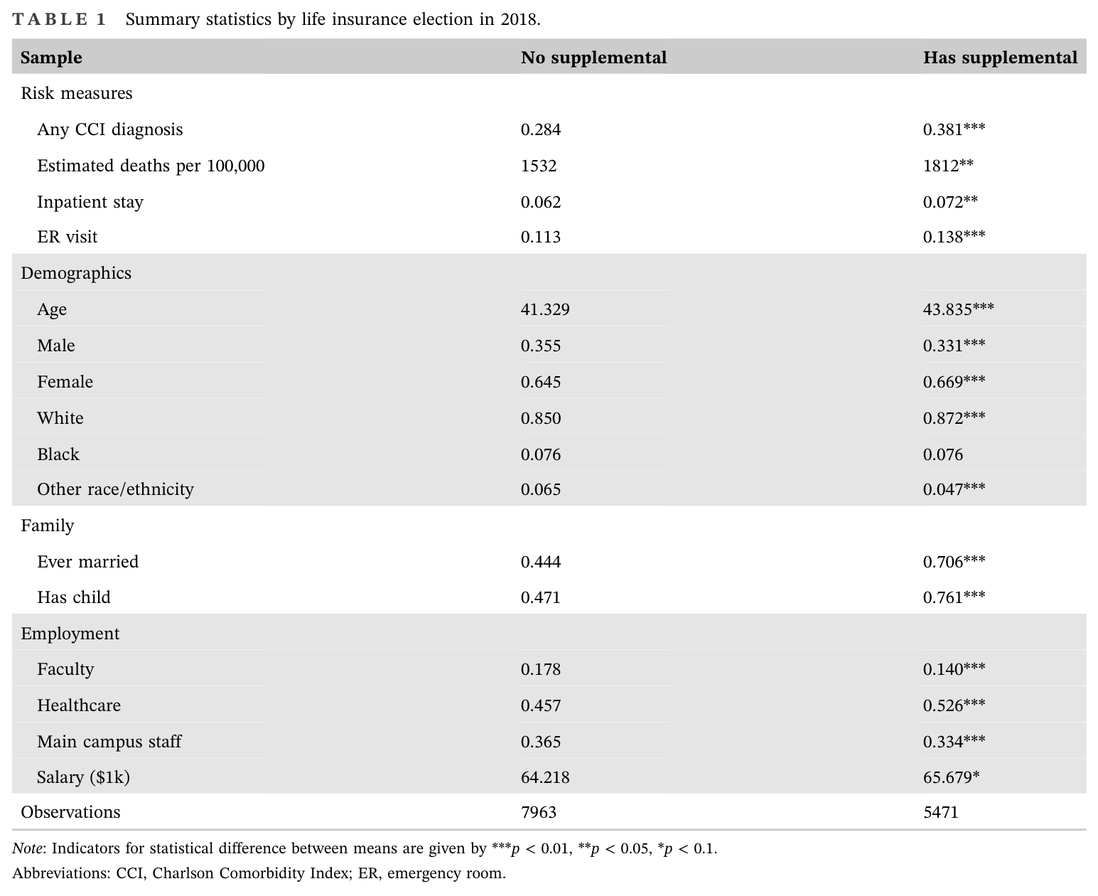
Table 1 presents the main summary statistics for 2018 separated by supplemental ESLI participation. The proportion of employees with a CCI diagnosis is higher for those with supplemental ESLI coverage (38.1%) than those without (28.4%) in 2018.³²

Furthermore, the probability of death is higher for those with supplemental coverage (1812 per 100,000) than those without supplemental coverage (1532 per 100,000). Consistent with the previous two metrics, those with supplemental ESLI coverage also are more likely to have an inpatient hospital stay and frequent the emergency room (ER).³³ Overall, these raw statistics point to adverse selection in supplemental ESLI. Nonetheless, the raw comparison does not account for differences in age or the primary demand determinants, which have the potential of explaining the differences.

Figure 3. Cause of death by age group

Cause of death by age group. Source: Centers for Disease Control and Prevention Mortality Multiple Cause‐of‐Death Data.

In addition to the differences in health, the table shows that the sample is predominately white, that a majority of the employees are female, and that healthcare workers constitute almost half of all employees. Individuals with supplemental ESLI are, on average, a few years older, less likely to be faculty, more likely to work in healthcare, and earn slightly more on average than those that do not have coverage.³⁴

The most pronounced difference is that individuals with coverage are more likely to be married or have children consistent with demand determinants for life insurance (Hong & Ríos‐Rull, 2012; Lewis, 1989).³⁵

Under half of the sample (40.7%) has supplemental coverage in 2018. Of those with supplemental ESLI in 2018, the average multiple of coverage was 2.7× salary, which translates into an average face value of $179,289.

Table 1. Summary statistics by life insurance election in 2018

6. EMPIRICAL MODELS

6.1. Positive correlation tests

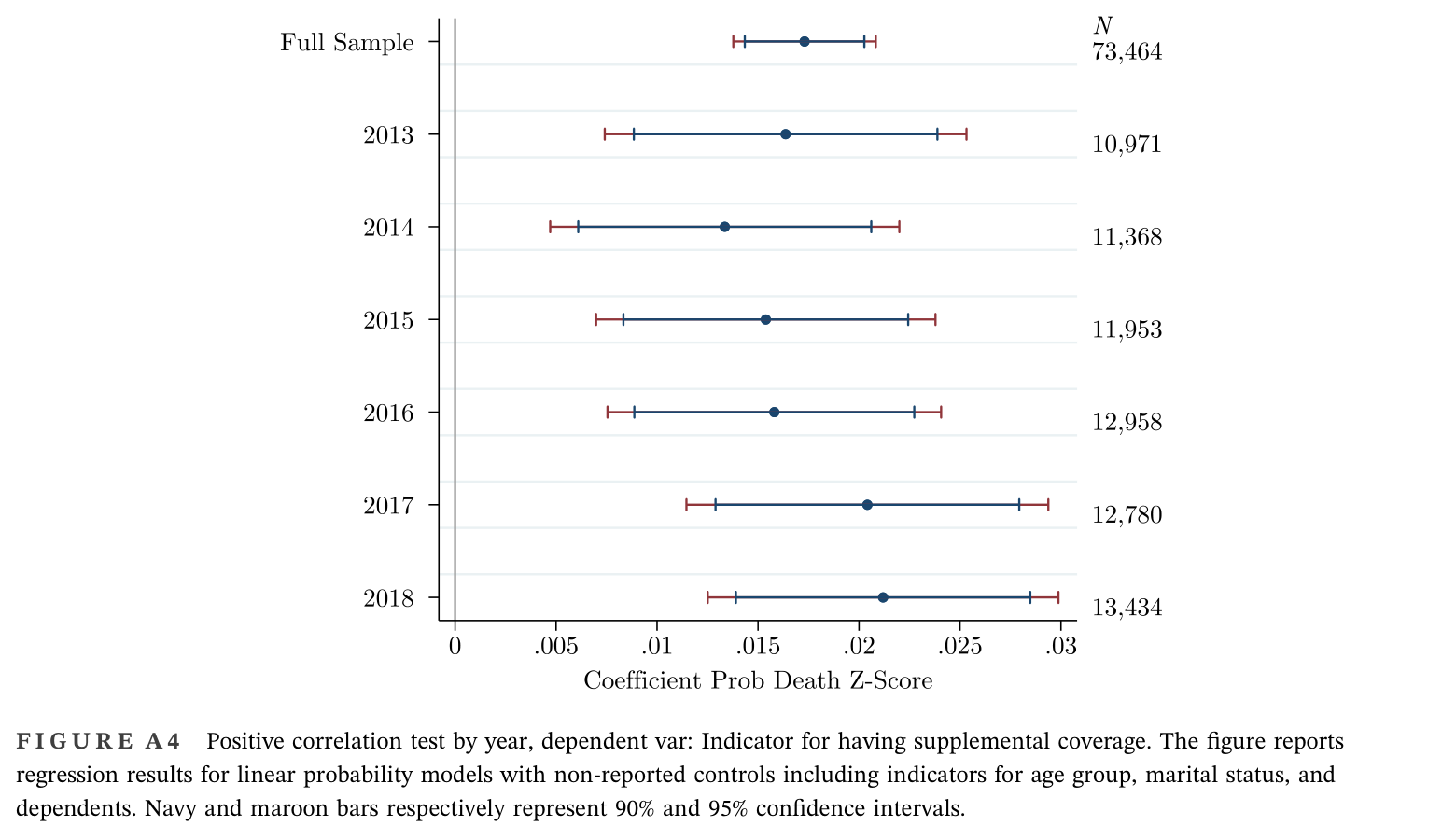
To determine the existence of adverse selection in the ESLI market, we use the commonly implemented positive correlation test (Cawley & Philipson, 1999; Chiappori & Salanie, 2000; Einav et al., 2010; Finkelstein & McGarry, 2006; Harris & Yelowitz, 2014). The model tests if individuals that are more likely to use insurance are also more likely to purchase coverage. A positive correlation indicates either the existence of moral hazard or adverse selection. However, moral hazard in life insurance is unlikely given the dire steps required to receive a payout along with policy exemptions for suicide.³⁶ Consequently, a “positive correlation” finding for supplemental ESLI can be interpreted as adverse selection.³⁷ The model is given by:

Equation (1):

where ${\mathit{S}\mathit{u}\mathit{p}\mathit{p}\mathit{l}\mathit{e}\mathit{m}\mathit{e}\mathit{n}\mathit{t}\mathit{a}\mathit{l}\mathit{E}\mathit{S}\mathit{L}\mathit{I}}_i$ represents either the decision to purchase any coverage (i.e., extensive margin) or the amount of coverage (i.e., intensive margin). ${\mathit{P}\mathit{r}\mathit{o}\mathit{b}\mathit{D}\mathit{e}\mathit{a}\mathit{t}\mathit{h}}_i$ is our constructed measure of an individual's probability of death converted to a Z ‐score (mean zero and standard deviation one). ${\mathit{A}\mathit{g}\mathit{e}\mathit{B}\mathit{i}\mathit{n}}_i$ is a vector of indicators for individual i 's age bin used by the life insurance company to determine an employee's premiums. By controlling for age bin, the specification compares individuals offered identical prices and allows for analysis within the risk class assigned by the insurance company (Einav & Finkelstein, 2011; He, 2009). Adverse selection resulting in increased premiums from a welfare perspective is only relevant for those individuals whose decision to purchase coverage or whose cost of coverage is influenced by an increased price due to adverse selection. In other words, the mortality risk of individuals that do not desire life insurance coverage—even at actuarially fair premiums—should not cause welfare loss. Therefore, following the work of Cawley and Philipson (1999) and Hedengren and Stratmann (2016) we include controls, $X_i$ , for the main demand‐side determinants of life insurance coverage—marital status, and children. Controlling for additional factors (e.g., gender, race, and employee position) in a positive correlation test is inappropriate as including these other variables would absorb some of the variation in the risk category that we are testing for.

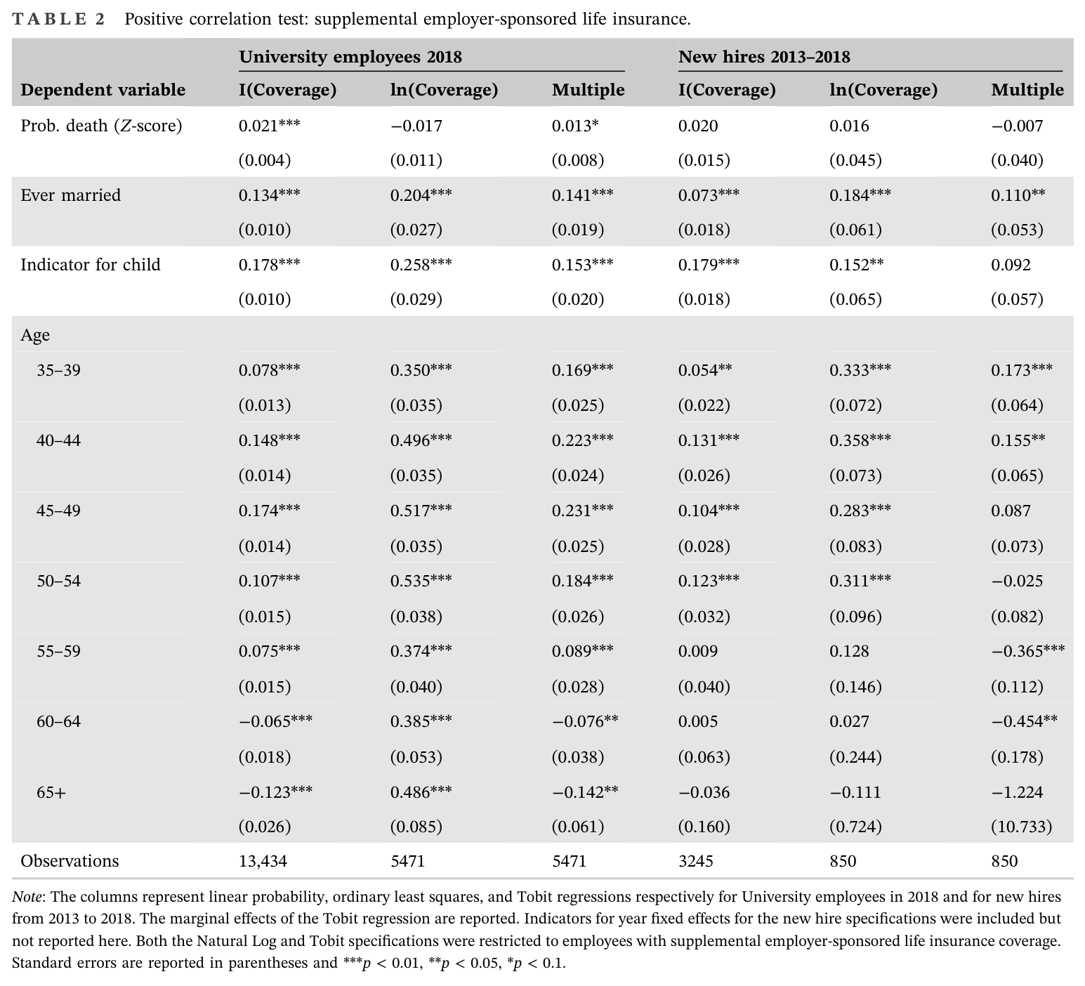
Table 2 presents the results of the positive correlation test for 2018.³⁸ The first column of the table shows a positive and statistically significant relationship between an employee's probability of death and whether the individual elects any supplemental life insurance coverage. This result indicates adverse selection on the extensive margin—whether to elect any coverage.³⁹

The second column of Table 2 uses the natural log of supplemental coverage as the dependent variable to estimate adverse selection on the intensive margin (i.e., how much coverage to elect conditional on having coverage). For employees with coverage, the results indicate that those with a higher probability of death did not elect more coverage than those with a lower probability of death. The cause of this lack of adverse selection finding on the intensive margin could be influenced by differential behavior by high and low earners as coverage is elected in multiples of annual salary. To explore this possibility, we present in the third column the marginal effect of a Tobit regression where the dependent variable is the multiple of salary bounded by one to five for employees with supplemental ESLI. The point estimate (marginal effect reported) on the probability of death is statistically significant and positive, indicating that employees at higher risk of death do elect higher multiples of coverage. Together, the log and multiple of salary specifications suggest lower amounts of adverse selection on the intensive margin for higher‐income employees who elected coverage.

The last three columns of the table report the results for the first observed elections of employees hired from 2013 to 2018. New employees are consequential for adverse selection because they may initially elect coverage without EOI. If they decline coverage in their first year, they must provide EOI if they ever wanted to elect supplemental coverage. Furthermore, given inertia in benefit elections, decisions regarding supplement ESLI made in the first year can significantly influence overall adverse selection. As shown in Table 2, there is no evidence of a statistically significant relationship between supplemental ESLI elections and mortality risk as measured by the probability of death metric. This lack of adverse selection among new hires likely results in lower overall adverse selection as employees are required to provide EOI for any coverage if they do not elect supplemental ESLI during their initial enrollment period.

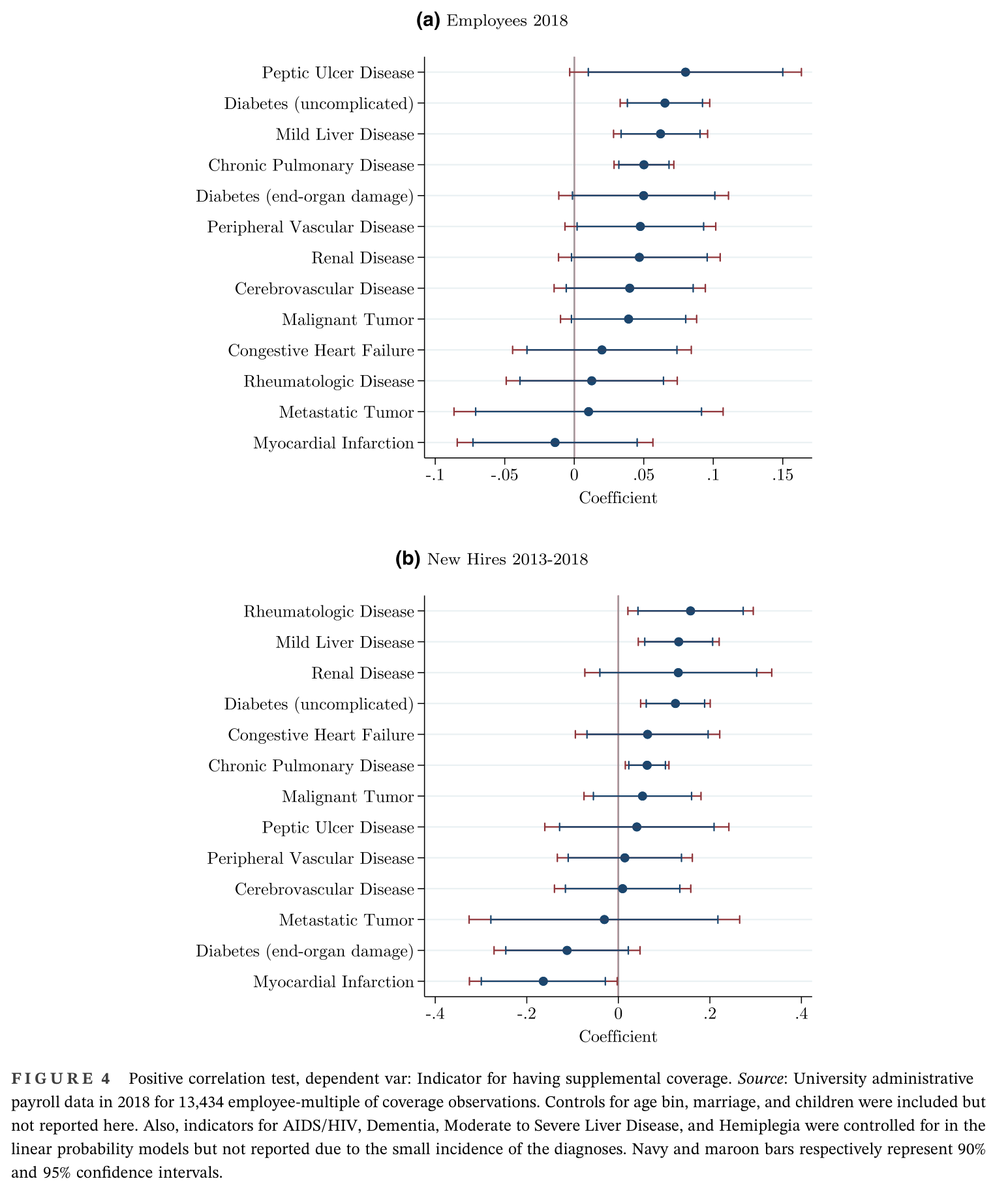
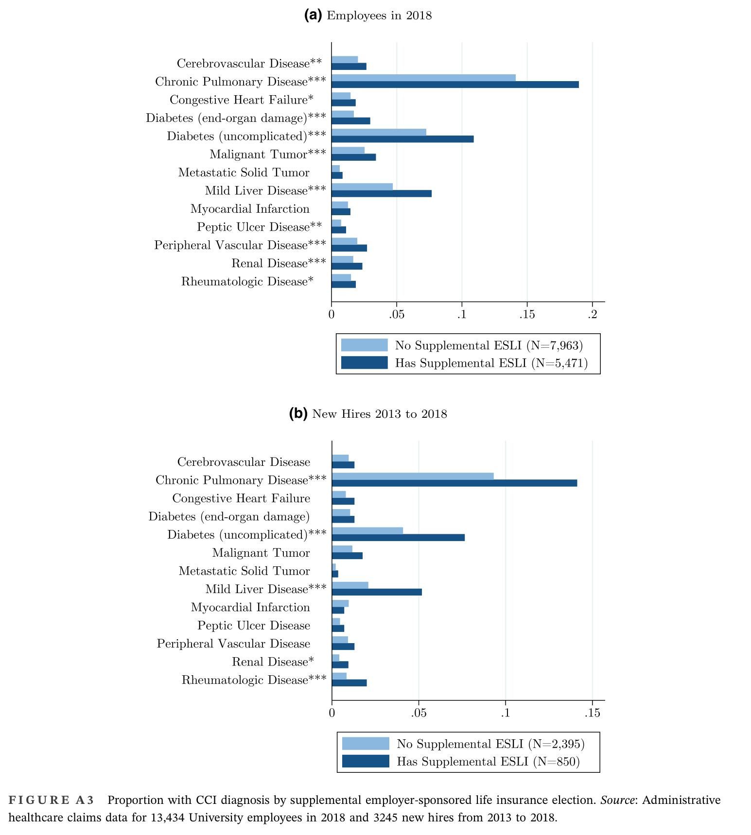
One potential concern with analysis using our probability of death measure is that the assumptions used to construct the CCI metric could be driving the results. To alleviate these concerns, in Figure 4, we present the results with indicators for the various CCI diagnoses as the main independent variables of interest rather than the probability of death. As illustrated, several diagnoses are positively correlated with electing life insurance coverage, including the three most prevalent diagnoses among university employees, Chronic Pulmonary Disease, Diabetes (uncomplicated), and Mild Liver Disease.⁴⁰ A similar pattern is observed for new hires but with fewer statistically significant coefficients, which suggests some adverse selection among the new hires.

Overall, these regressions indicate the presence of adverse selection mainly coming from the extensive margin.

6.2. Heterogeneity analysis

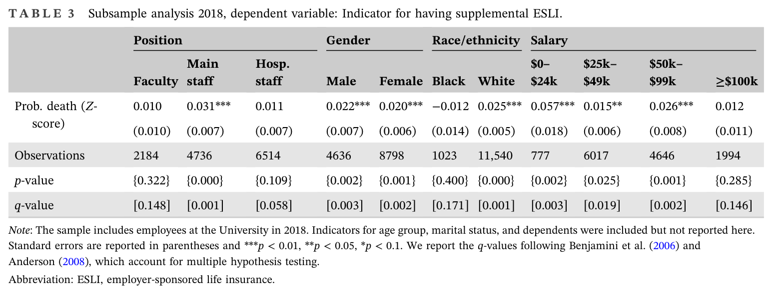
In addition to analyzing the existence of adverse selection, we also explore which groups are more likely to take advantage of the asymmetric information. Table 3 presents the results of several subsample extensive margin analyses based on employment type, demographics, and salary. To correct for the potential issues associated with multiple hypothesis testing, we follow Benjamini et al. (2006) and Anderson (2008) to calculate and report q‐values—the minimum false discovery rate (FDR).⁴¹

The estimates indicate that main campus staff exhibit statistically significant adverse selection, whereas faculty and healthcare staff do not at the ten‐percent level. There does not seem to be any meaningful differences in adverse selection by gender. The table also shows that white employees adversely select coverage, whereas there is no evidence of adverse selection for African–American employees. Perhaps most importantly, individuals with the lowest income have the largest point estimate indicative of adverse selection, whereas the highest earners point estimate is significantly smaller and statistically insignificant. Given that coverage is elected in multiples of salary, the lack of adverse selection by the highest earners is particularly important for the overall functionality of the market.

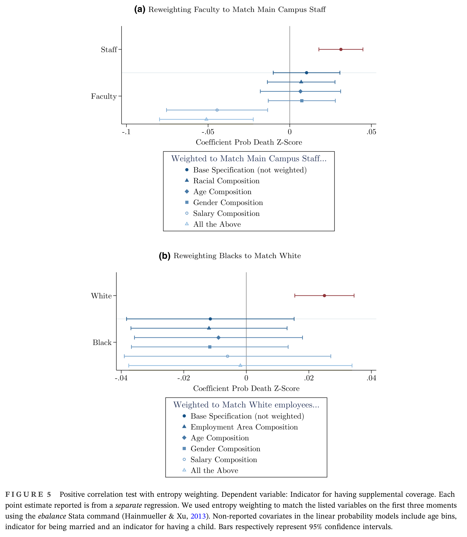
To explore the differences in adverse selection, we use entropy weighting to see which, if any of the observable differences, can explain the results (Hainmueller, 2012). Specifically, we weight the sample of faculty members to match the characteristics (age, gender, race/ethnicity, and salary) of main campus staff.⁴² Figure 5a presents the results of reweighting on these characteristics. As shown, reweighting the sample does not explain the difference in findings for adverse selection and if anything exacerbates the difference in the estimated results of the correlation between probability of death and supplemental ESLI participation. Similarly in Figure 5b, we reweight the sample of black employees to reflect the characteristics (age, gender, employment area, and salary) of white employees, but once again the reweighting does not explain the difference. One possible explanation for the lack of adverse selection for faculty and high earners is higher levels of risk aversion leading to advantageous selection. In the spirit of Finkelstein and McGarry (2006), we use preventive care visits to proxy for risk aversion to determine its influence on the results from the heterogeneity analysis.⁴³

Table 2. Positive correlation test: supplemental employer‐sponsored life insurance

Figure 4. Positive correlation test, dependent var: Indicator for having supplemental coverage

Positive correlation test, dependent var: Indicator for having supplemental coverage. Source: University administrative.

We label an employee as being risk averse if they have preventive care visits that exceed the median for their gender and age group. Nonetheless, this metric of risk aversion is largely uncorrelated with supplemental ESLI coverage (ρ = 0.02) and also largely uncorrelated with probability of death (ρ = 0.01). Consequently, even though advantageous selection could be causing the heterogeneous results, our limited metric for risk aversion does not explain the difference.

6.3. Robustness to an alternative risk metric

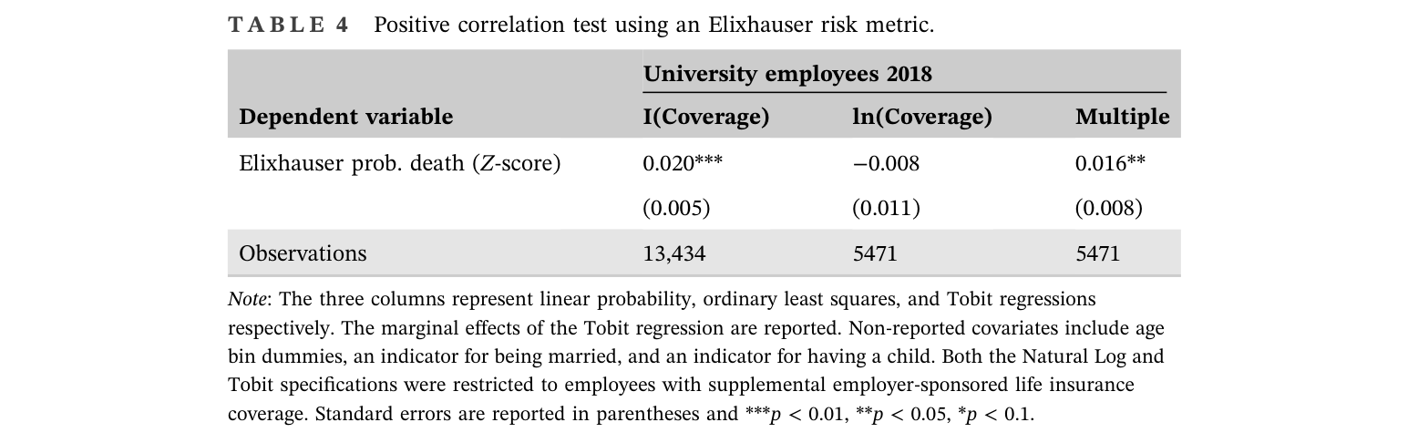
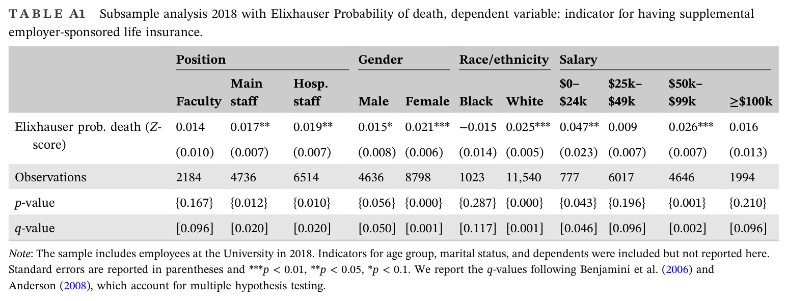
As a robustness test, we use the Elixhauser comorbidity score as an alternative risk metric. Similar to the CCI, the Elixhauser comorbidity score (Elixhauser et al., 1998) identifies major diagnoses that are correlated with adverse health outcomes, particularly in‐hospital mortality, and van Walraven et al. (2009) details a method to construct a single metric that captures mortality risk.⁴⁴

The Walraven metric ranges from −19 to 89 and maps into a probability of death in hospital metric that is arguably highly correlated with an individual's overall probability of death. We calculate a Z‐ score for an individual's probability of death and use this metric as the independent variable in the regression analysis presented in Table 4.⁴⁵

As shown, the results and consistent with the previous findings indicating adverse selection on the extensive margin and some evidence of higher risk individuals electing higher multiples of coverage.⁴⁶

6.4. Response to diagnoses

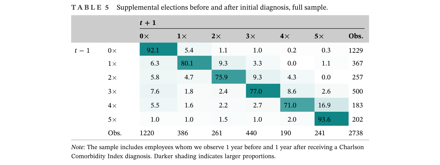
To analyze how individuals respond to health information, we compare supplemental ESLI elections around the time of diagnosis. Table 5 presents a transition matrix that looks at elections the year before (t − 1) an employee gets a new CCI diagnosis compared to their elections 1 year after their diagnosis (t + 1). Overall, there are 2738 employees whom we observe 1 year before and 1 year after receiving a CCI diagnosis. The table shows that most employees (84.9%) do not change their supplemental ESLI elections even after receiving a diagnosis. Nonetheless, 9.8% of employees increased coverage potentially consistent with adverse selection. Perhaps surprisingly, 5.3% decreased coverage following a diagnosis that significantly impacted their projected mortality. Most of the employees that decreased coverage decided to altogether drop supplemental ESLI rather than decrease coverage on the intensive margin. One explanation for the decreased coverage following a diagnosis is an increased need for disposable income due to the illness. Nonetheless, supplemental ESLI represents a relatively small cost, which decreases the likelihood that disposable income is the main factor.⁴⁷

Overall, total multiples of salary of supplemental ESLI increased by 1.7% (from 4123 to 4193 multiples), which could be caused by adverse selection or merely increased desire for coverage as employees age.

Table 3. Subsample analysis 2018, dependent variable: Indicator for having supplemental ESLI

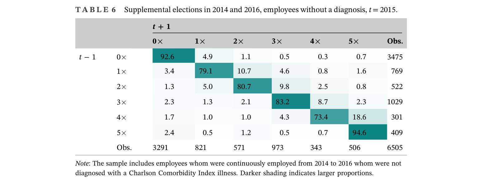
To understand if the behavior of these employees who received a diagnosis is atypical, we also present the transition matrix for employees who did not receive a CCI diagnosis from 1 year to the next (i.e., a placebo group). Specifically, we look at the response of employees from 2014 to 2016 who were not diagnosed with a CCI illness in the 3‐year window.⁴⁸

As shown in Table 6, 87.8% of the employees did not change coverage, 9.7% increased coverage, and 2.5% decreased coverage. The percentage of employees that increased coverage is nearly identical to the full sample of those that received a diagnosis.⁴⁹

In addition, the proportion of employees that decided to drop coverage altogether is lower than observed for those that received a negative diagnosis. Overall, total multiples of salary of supplemental ESLI increased by 7.8%, significantly more than the increase observed for those that received a diagnosis.

Figure 5. Positive correlation test with entropy weighting

Positive correlation test with entropy weighting. Dependent variable: Indicator for having supplemental coverage. Each.

Table 4. Positive correlation test using an Elixhauser risk metric

Table 5. Supplemental elections before and after initial diagnosis, full sample

Table 6. Supplemental elections in 2014 and 2016, employees without a diagnosis, t = 2015

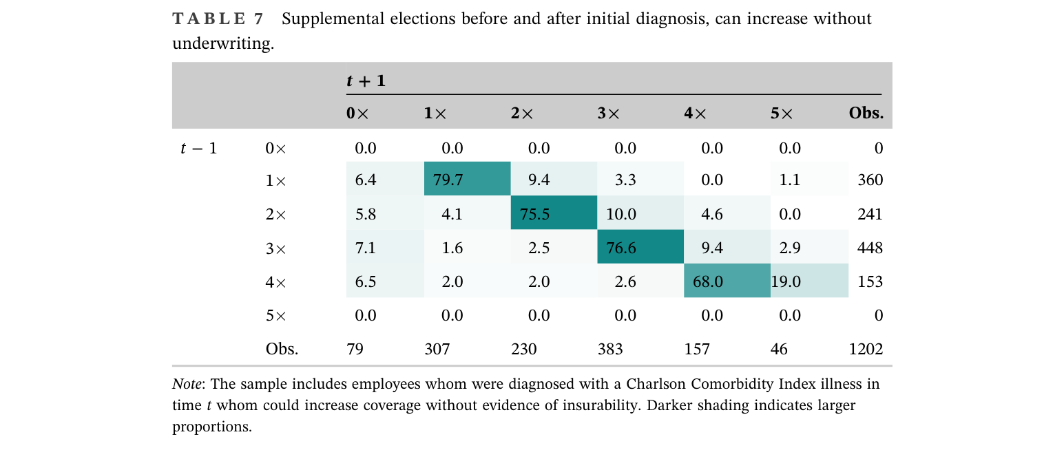
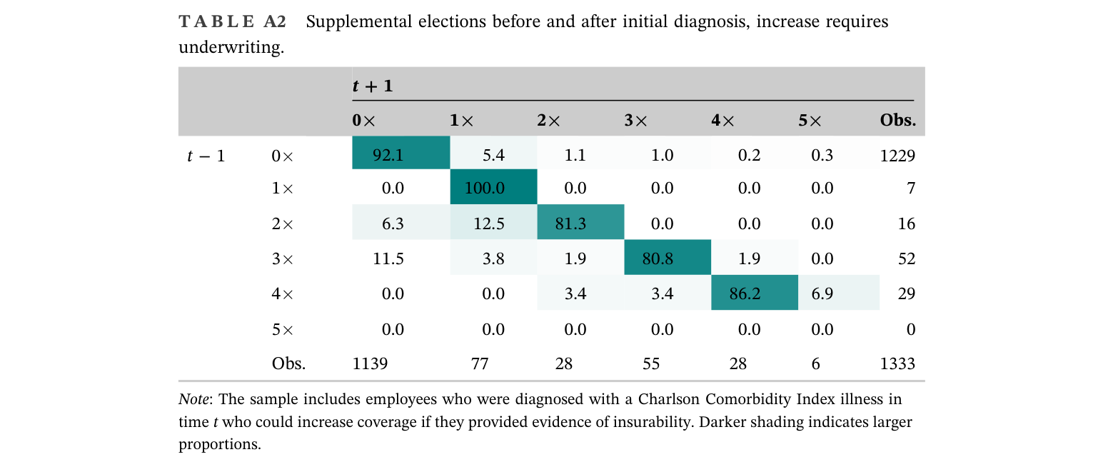
One possible explanation why more employees did not increase coverage after receiving a diagnosis is that many individuals would have to provide EOI to increase coverage. To abstract away from this concern, we present a transition matrix in Table 7 that restricts the sample to employees that could have increased coverage without providing EOI. As illustrated, there is a slight increase in the proportion of employees that increased coverage, suggesting that some employees might have increased coverage if allowed to do so without EOI.⁵⁰

Nonetheless, there is a 0.9% overall decrease in the total multiples of salary in coverage in the year following the diagnosis for those that could increase coverage without EOI, in large part driven by individuals that drop coverage altogether. These raw statistics suggest that overall changes in coverage following a diagnosis are unlikely to have a meaningful overall impact on adverse selection.

To more formally test if employees differentially increase supplemental ESLI in response to negative health information, we estimate the following regression.

Equation (2):

is a dynamic measure of the CCI index, and $AgeBi{n}_{it}$

once again includes indicators for the age bins used to price the policies. The vector $X_{it}$

includes dynamic measures of being married and having a child as derived from benefit elections. Individual and time fixed effects are given respectively by ${\alpha }_i$

and ${\delta }_t$

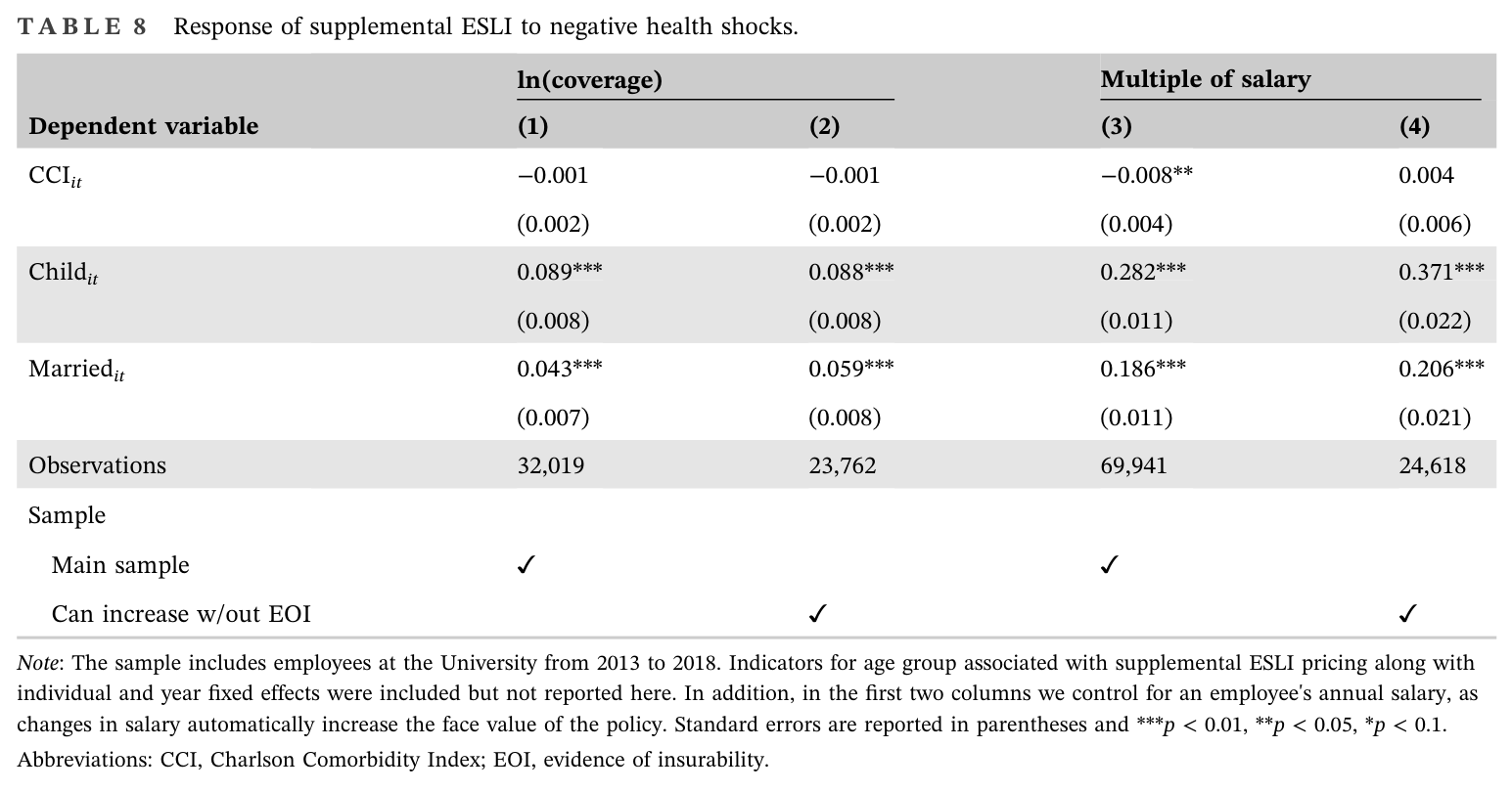
Table 8 first presents the estimation results with the natural log of coverage as the dependent variable. The first column contains the primary sample of employees, whereas the second column only includes observations where the employee could have increased coverage without providing EOI in the previous year. In both specifications, there is no statistically significant positive correlation between increased mortality risk, proxied for by the CCI, and supplemental ESLI coverage. The last two columns of the table present similar findings for a specification that uses the multiple of coverage as the dependent variable.⁵¹

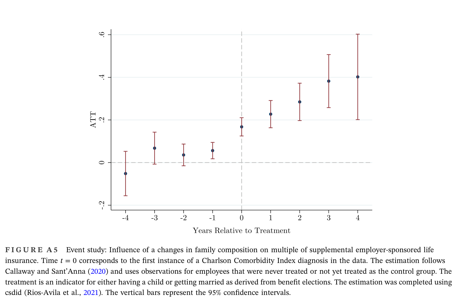
Importantly, in each of the specifications, family composition changes significantly impact coverage levels, indicating that employees are aware that they can increase coverage.⁵² In addition, we use an event study framework to estimate the influence of a CCI diagnosis on supplemental ESLI.

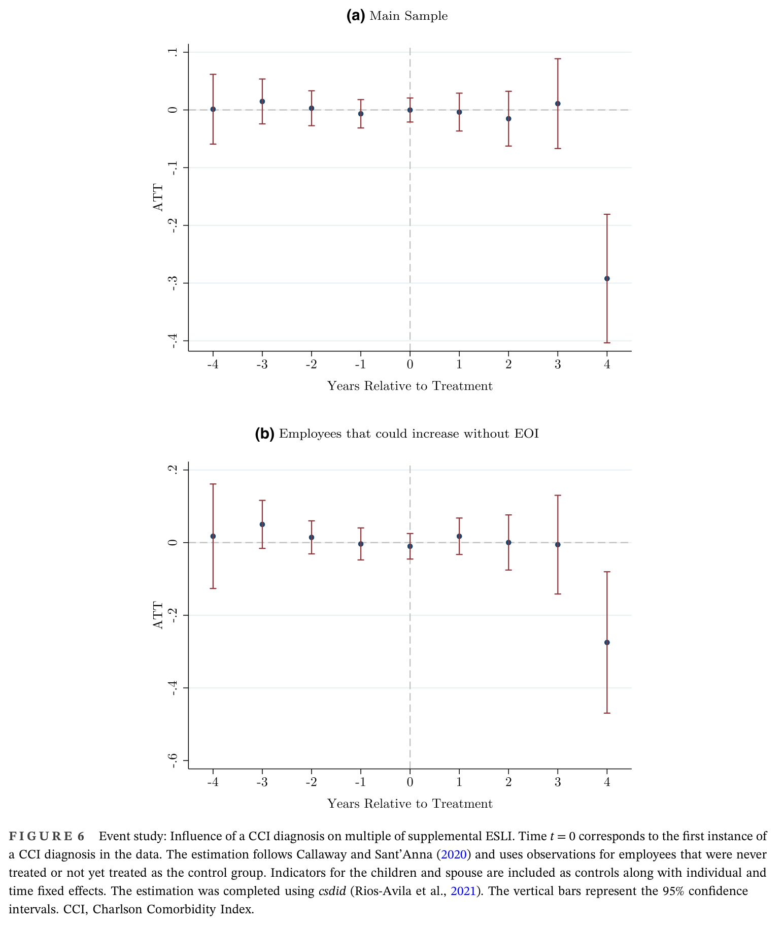
Following the work of Callaway and Sant’Anna (2020) we estimate the group‐time average treatment effects (e.g., all individuals first diagnosed in 2014 represent a single group) and then aggregate the group‐time effects to get the average treatment effects for the years surrounding the initial diagnosis. We use observations that are never treated as well as those that are not yet treated as the control group. Figure 6a plots the average treatment on the treated (ATT) in the years surrounding the diagnosis. As illustrated, there is no evidence of changes to life insurance elections for this sample. Figure 6b shows that the main finding of no statistically significant response remains unchanged when the sample is restricted to employees that could increase coverage without providing EOI.⁵³ One potential explanation for the lack of increase following a diagnosis is that employees do not understand that they may increase coverage without providing EOI. Another explanation is the well‐documented levels of inertia in benefit elections through an employer (e.g., Harris & Yelowitz, 2017). In theory, significant diagnoses have the potential to incentivize greater understanding of and attention to life insurance options and thus overcome inertia and the lack of salience. However, in practice, employees do not on average, take advantage of the ability to increase coverage, which likely explains the lack of a death spiral in supplemental ESLI.

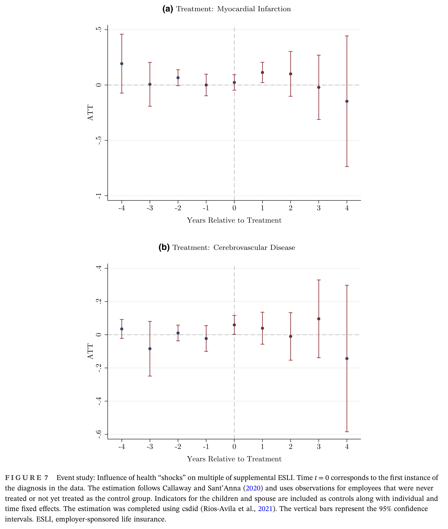
Yet another explanation is that these diagnoses are not health “shocks” rather a confirmation of known health issues. For example, an individual diagnosed with Chronic Obstructive Pulmonary Disease (COPD) would have already experienced significant respiratory issues, and the diagnosis might only represent a marginal increase in mortality information. On the other hand, an individual who has a heart attack or stroke likely has a much larger update to their expectations on mortality. To test this hypothesis, we analyze employee responses to myocardial infarctions and cerebrovascular disease (e.g., stroke) separately. As shown in Figure 7, in the year following a heart attack or the year of a cerebrovascular disease diagnosis, individuals increased their multiple of supplemental ESLI. Nonetheless, even though there are statistically significant point estimates the increases are economically insignificant.⁵⁴

Table 7. Supplemental elections before and after initial diagnosis, can increase without

7. INFLUENCE ON EXPECTED COSTS AND PREMIUMS

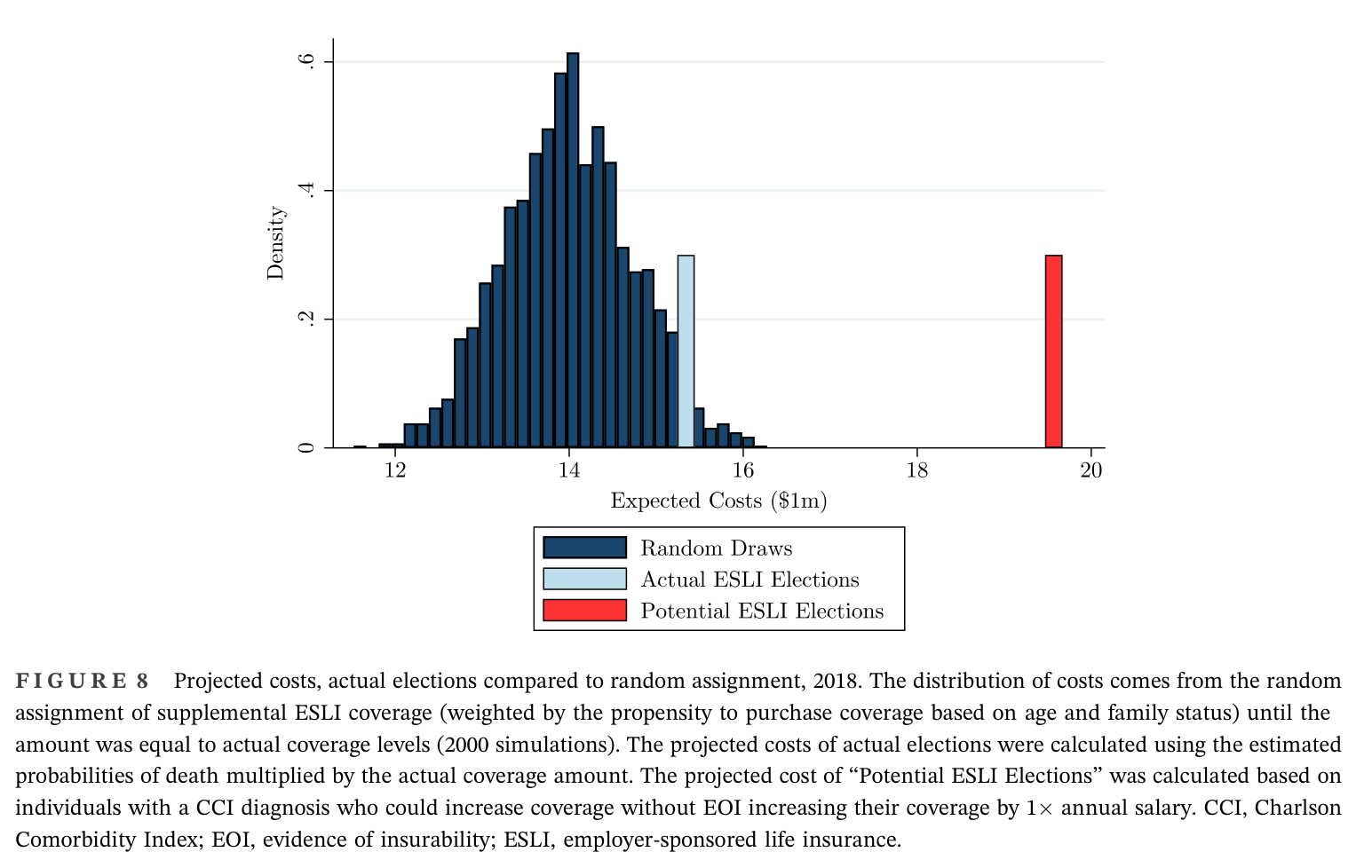
To better understand the cumulative influence of adverse selection on premiums in the market, we compare the expected costs of the pool of insured employees to randomly drawn samples of employees. We randomly assign the median multiple of coverage conditional on having supplemental ESLI, 3× annual salary, to employees until the total dollar amount of life insurance coverage equals the actual coverage in 2018. To account for differences in demand determinants, we weight observations by the proportion of individuals of a given age and family status (i.e., has children or married)

that have coverage when drawing the random samples.⁵⁵ Figure 8 compares the expected costs of the random samples to the expected cost of the actual sample of insured employees using our constructed metric for the probability of death. Figure 8 presents the overall results and indicates that the sample of employees that purchased coverage has costs in the 97.0%, indicative of adverse selection. Another way of describing the results is that adverse selection caused the actual expected costs to be 9.7% higher than the median of the simulated costs from the random assignment of benefits.

To visualize how much larger expected costs could have been, we also plot the “potential” expected cost if employees with a CCI diagnosis, who also could have increased coverage without EOI, would have increased their elections by 1× their annual salary.⁵⁶

As shown, the “potential” expected costs are 40.0% higher than the median of the simulated costs. Consistent with the main analysis, this figure indicates that the amount of adverse selection is far below the potential since individuals generally did not take advantage of the ability to increase coverage following a negative health shock.

One important caveat is that the expected costs illustrated in Figure 8 are significantly higher than the premiums the life insurance company received for the actual policies issued. There are a few possible explanations for the difference.

First, as mentioned earlier, the probability of death metric is likely elevated because employed individuals are—all else equal—in better health than the general population (Roelfs et al., 2011). Consequently, the mortality risk assigned for those with a CCI diagnosis is likely too high, which increases the expected costs. Second, and perhaps more importantly, employees might exit (e.g., retire early) the University when their health deteriorates. Given the conditional nature of ESLI, in most cases, the policy would lapse for the separated employee, and the life insurance company would not be required to pay the decedent's dependents.⁵⁷

Nonetheless, the above projections are still informative for quantifying the relative influence of adverse selection and gauging potential adverse selection.

Table 8. Response of supplemental ESLI to negative health shocks

In canonical models of life insurance pricing, increases in expected costs directly translate into increased premiums. Increased premiums due to adverse selection result in a lower quantity demanded and welfare loss. To get a sense of the magnitude of the influence of any increased premiums on the market, we estimate the impact of price changes on both extensive margin participation and intensive margin decisions of supplemental ESLI coverage levels. To identify the model, we use discontinuous increases in premiums associated with the age bins used to price supplemental ESLI policies at the University. The discontinuous jumps in ESLI pricing do not accurately reflect actuarial adjustments for a 1‐year increase in age, and we argue that they can be used as exogenous price variation. For example, an individual who ages from 44 to 45 experiences a slight (almost negligible) increase in the probability of death, whereas the ESLI premium increases by 50%.

Figure 6. Event study: Influence of a CCI diagnosis on multiple of supplemental ESLI

Event study: Influence of a CCI diagnosis on multiple of supplemental ESLI. Time t = 0 corresponds to the first instance of.

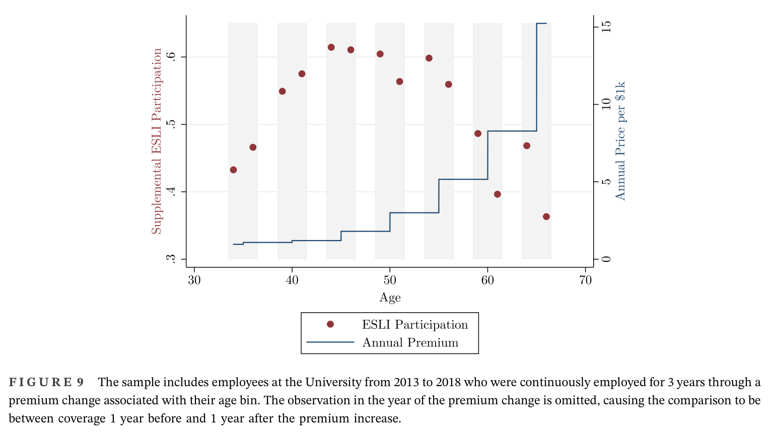
For this estimation, we use a sample of individuals who were employed continuously for 3 years surrounding a premium change (1 year before, the year of, and 1 year after the premium change). We then exclude the observation for the year of the premium increase for the employee and thus compare coverage in the year prior with the year following the increased premium.⁵⁸ Figure 9 plots supplemental ESLI participation for this sample by age and shows that supplemental ESLI participation generally decreases with the increased premiums. Nonetheless, the earliest two premium increases show increased participation potentially due to changes in family structure, which could increase the demand for life insurance. At the same time, the decreases in the later periods might be caused by decreased need for life insurance coverage as dependents become more independent. Consequently, in the empirical specification below, we control for the main demand‐side determinants of life insurance coverage.

Figure 7. Event study: Influence of health “shocks” on multiple of supplemental ESLI

Event study: Influence of health “shocks” on multiple of supplemental ESLI. Time t = 0 corresponds to the first instance of.

Figure 8. Projected costs, actual elections compared to random assignment, 2018

Projected costs, actual elections compared to random assignment, 2018. The distribution of costs comes from the random.

Figure 9. Supplemental ESLI participation and premiums by age

The sample includes employees at the University from 2013 to 2018 who were continuously employed for 3 years through a premium change associated with their age bin. The observation in the year of the premium change is omitted, causing the comparison to be between coverage 1 year before and 1 year after the premium increase.

The estimation is given by:

Equation (3):

where ${\mathit{S}\mathit{u}\mathit{p}\mathit{p}\mathit{l}\mathit{e}\mathit{m}\mathit{e}\mathit{n}\mathit{t}\mathit{a}\mathit{l}\mathit{E}\mathit{S}\mathit{L}\mathit{I}}_{it}$ is either an indicator for having coverage or the log of coverage depending on the specification for employee i at time t . ${\mathit{L}\mathit{o}\mathit{g}\mathit{P}\mathit{r}\mathit{e}\mathit{m}\mathit{i}\mathit{u}\mathit{m}}_{it}$ is the natural log of premiums per $1000 in coverage, and $X_{it}$ is a vector containing dynamic measures of salary, an indicator for the presence of a child, and an indicator for the presence of a spouse.

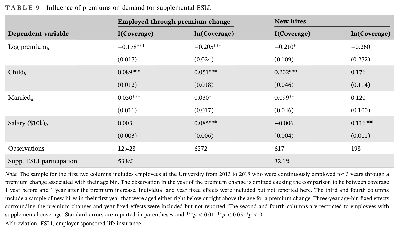
Table 9 presents the results of the demand regressions. The estimates in the first and second columns respectively indicate that a 10% in premiums results in a 1.78% point decrease in supplemental ESLI participation and a 2.05% decrease in the level of supplemental ESLI coverage. These results indicate that employees have a very inelastic demand for life insurance coverage with likely causes including inertia, salience, and the small budget share. Consequently, any premium increase that resulted from adverse selection likely did not cause economically significant welfare loss.

Nonetheless, higher premiums due to adverse selection could arguably impact new hires more than existing employees as premiums are more salient and inertia from previous elections is not a concern. The last two columns of Table 9 present the results of regressions that analyze ESLI election differences for those hired at an ages surrounding a premium change (e.g., compare those aged 44 and 46) while controlling for 3‐year age fixed effects surrounding the change.⁵⁹ The results indicate a slightly larger—but still inelastic—extensive margin response compared to the panel regression of workers employed through a premium change, but no statistically significant response on the intensive margin.

8. CONCLUSION

Supplemental ESLI provides a textbook example of a market that could have ruinous adverse selection. At the University analyzed in this study, premiums are community‐rated, coverage is mainly guaranteed issue, individuals can increase coverage after a negative health diagnosis, and there exists a competitive term life insurance market that offers lower premiums to healthy individuals. All these features of supplemental ESLI should exacerbate adverse selection.

Table 9. Influence of premiums on demand for supplemental ESLI

Consistent with these features, we find adverse selection using the widely‐implemented positive correlation test. Nonetheless, we find that adverse selection is significantly lower than it could have been because high earners did not exhibit adverse selection, and individuals diagnosed with a CCI diagnosis did not generally increase coverage. Altogether, the simulation results imply that adverse selection likely only caused premiums to be elevated by around 10%. In conjunction with the study's finding that employees have highly inelastic demand for supplemental ESLI, this result points to minimal welfare loss from adverse selection.

There are several reasons why this market that is ripe for adverse selection does not result in ruinous market failure, including well‐documented inertia in life insurance elections, lack of salience in the ability to increase coverage, and the relative ease of electing ESLI compared to the underwriting required in the term life insurance market. Furthermore, life insurance companies are not overly concerned about adverse selection in this market due to both the inelastic demand and, perhaps more importantly, the conditional nature of the coverage. In other words, even if those in worse health purchase more coverage or ramp up coverage, many of them will likely leave employment and lose their coverage.

ACKNOWLEDGMENTS

The project was supported by the National Center for Advancing Translational Sciences, National Institutes of Health, through Grant UL1TR001998. The content is solely the responsibility of the authors and does not necessarily represent the official views of the National Institutes of Health. We thank Bibek Adhikari, David Agrawal, Tom Ahn, Chris Bollinger, Charles Courtemanche, Anthony Creane, John Garen, Kristine Hankins, Jeremiah Harris, William Hoyt, Conor Lennon, Frank Scott, and James Ziliak for helpful comments and Matthijs Schendstok and Lydia Tetteh for research assistance. We also thank the co‐editor and anonymous referees for their helpful suggestions.

5. DATA AVAILABILITY STATEMENT

The code and non‐confidential portion of the data that support the findings of this study are openly available at http://doi.org/10.3886/E188604V3, See Harris et al., 2023.

ORCID

Aaron Yelowitz https://orcid.org/0000-0001-8847-1437

References

American Council of Life Insurers (2021) 2021 Life Insurance Fact Book. Available from: https://www.acli.com/-/media/acli/files/fact-books-public/2021lifeinsurersfactbook.pdf - Anderson, M.L. (2008) Multiple inference and gender differences in the effects of early intervention: a reevaluation of the Abecedarian, Perry Preschool, and early training projects. Journal of the American Statistical Association , 103(484), 1481–1495. Available from: https://doi.org/10.1198/016214508000000841 - Barsky, R.B., Juster, F.T., Kimball, M.S. & Shapiro, M.D. (1997) Preference parameters and behavioral heterogeneity: an experimental approach in the health and retirement study. Quarterly Journal of Economics , 112(2), 537–579. Available from: https://doi.org/10.1162/003355397555280 - Benjamini, Y., Krieger, A.M. & Yekutieli, D. (2006) Adaptive linear step‐up procedures that control the false discovery rate. Biometrika , 93(3), 491–507. Available from: https://doi.org/10.1093/biomet/93.3.491 - Bernheim, B.D., Forni, L., Gokhale, J. & Kotlikoff, L.J. (2003) The mismatch between life insurance holdings and financial vulnerabilities: evidence from the health and retirement study. The American Economic Review , 93(1), 354–365. Available from: https://doi.org/10.1257/000282803321455340 - Brown, J.R. & Goolsbee, A. (2002) Does the internet make markets more competitive? Evidence from the life insurance industry. Journal of Political Economy , 110(3), 481–507. Available from: https://doi.org/10.1086/339714 - Buchmueller, T. & Dinardo, J. (2002) Did community rating induce an adverse selection death spiral? Evidence from New York, Pennsylvania, and Connecticut. The American Economic Review , 92(1), 280–294. Available from: https://doi.org/10.1257/000282802760015720 - Callaway, B. & Sant’Anna, P.H.C. (2020) Difference‐in‐differences with multiple time periods. Journal of Econometrics , 225(2), 200–230. Available from: https://doi.org/10.1016/j.jeconom.2020.12.001 - Cardon, J.H. & Hendel, I. (2001) Asymmetric information in health insurance: evidence from the National Medical Expenditure Survey. The RAND Journal of Economics , 32(3), 408–427. - Cawley, J. & Philipson, T. (1999) An empirical examination of information barriers to trade in insurance. The American Economic Review , 89(4), 827–846. Available from: https://doi.org/10.1257/aer.89.4.827 - Chandra, A., Gruber, J. & McKnight, R. (2014) The impact of patient cost‐sharing on low‐income populations: evidence from Massachusetts. Journal of Health Economics , 33, 57–66. Available from: https://doi.org/10.1016/j.jhealeco.2013.10.008 - Charlson, M.E., Pompei, P., Ales, K.L. & MacKenzie, C.R. (1987) A new method of classifying prognostic comorbidity in longitudinal studies: development and validation. Journal of Chronic Diseases , 40(5), 373–383. Available from: https://doi.org/10.1016/0021-9681(87)90171-8 - Chaudhry, S., Jin, L. & Meltzer, D. (2005) Use of a self‐report‐generated Charlson Comorbidity Index for predicting mortality. Medical Care , 43(6), 607–615. Available from: https://doi.org/10.1097/01.mlr.0000163658.65008.ec - Chiappori, P.‐A. & Salanie, B. (2000) Testing for asymmetric information in insurance markets. Journal of Political Economy , 108(1), 56–78. Available from: https://doi.org/10.1086/262111 Conning, Inc. (2014) 2014 Life‐Annuity Consumer Markets Annual. Cutler, D.M. (2002) Health care and the public sector. Handbook of Public Economics , 4, 2143–2243. - Cutler, D.M., Finkelstein, A. & McGarry, K. (2008) Preference heterogeneity and insurance markets: explaining a puzzle of insurance. The American Economic Review , 98(2), 157–162. Available from: https://doi.org/10.1257/aer.98.2.157 - Cutler, D.M. & Reber, S.J. (1998) Paying for health insurance: the trade‐off between competition and adverse selection. Quarterly Journal of Economics , 113(2), 433–466. Available from: https://doi.org/10.1162/003355398555649 De Meza, D. & Webb, D.C. (2001) Advantageous selection in insurance markets. The RAND Journal of Economics , 32(2), 249–262. Available from: https://doi.org/10.2307/2696408 Durham, A. (2016) 2016 Insurance Barometer Study . LIMRA. - Einav, L., Finkelstein, A. & Cullen, M.R. (2010) Estimating welfare in insurance markets using variation in prices. Quarterly Journal of Economics , 125(3), 877–921. Available from: https://doi.org/10.1162/qjec.2010.125.3.877 Einav, L. & Finkelstein, A. (2011) Selection in insurance markets: theory and empirics in pictures. The Journal of Economic Perspectives , 25(1), 115–138. Available from: https://doi.org/10.1257/jep.25.1.115 Elixhauser, A., Steiner, C., Harris, D.R. & Coffey, R.M. (1998) Comorbidity measures for use with administrative data. Medical Care , 36(1), 8–27. Available from: https://doi.org/10.1097/00005650-199801000-00004 - Fang, H., Keane, M.P. & Silverman, D. (2008) Sources of advantageous selection: evidence from the Medigap insurance market. Journal of Political Economy , 116(2), 303–350. Available from: https://doi.org/10.1086/587623 Federal Insurance Office, U.S. Department of the Treasury (2020) Annual report on the insurance industry. - Finkelstein, A. & Poterba, J. (2004) Adverse selection in insurance markets: policyholder evidence from the UK annuity market. Journal of Political Economy , 112(1), 183–208. Available from: https://doi.org/10.1086/379936

Finkelstein, A. & McGarry, K. (2006) Multiple dimensions of private information: evidence from the long‐term care insurance market. The American Economic Review , 96(4), 938–958. Available from: https://doi.org/10.1257/aer.96.4.938 Geruso, M., Layton, T.J., McCormack, G. & Shepard, M. (2023) The two margin problem in insurance markets. The Review of Economics and Statistics , 105(2), 237–257. Available from: https://doi.org/10.1162/rest_a_01070 Gutacker, N., Siciliani, L., Moscelli, G. & Gravelle, H. (2016) Choice of hospital: which type of quality matters? Journal of Health Economics , 50, 230–246. Available from: https://doi.org/10.1016/j.jhealeco.2016.08.001 Hainmueller, J. (2012) Entropy balancing for causal effects: a multivariate reweighting method to produce balanced samples in observational studies. Political Analysis , 20(1), 25–46. Available from: https://doi.org/10.1093/pan/mpr025 Hainmueller, J. & Xu, Y. (2013) Ebalance: a Stata package for entropy balancing. Journal of Statistical Software , 54(7), 1–18. Available from: https://doi.org/10.18637/jss.v054.i07 Halek, M. & Eisenhauer, J.G. (2001) Demography of risk aversion. Journal of Risk and Insurance , 68, 1–24. Available from: https://doi.org/10.2307/2678130 - Handel, B.R. (2013) Adverse selection and inertia in health insurance markets: when nudging hurts. The American Economic Review , 103(7), 2643–2682. Available from: https://doi.org/10.1257/aer.103.7.2643 Harris, T.F. & Yelowitz, A. (2014) Is there adverse selection in the life insurance market? Evidence from a representative sample of purchasers. Economics Letters , 124(3), 520–522. Available from: https://doi.org/10.1016/j.econlet.2014.07.029 Harris, T.F. & Yelowitz, A. (2017) Nudging life insurance holdings in the workplace. Economic Inquiry , 55(2), 951–981. Available from: https://doi.org/10.1111/ecin.12390 Harris, T., Yelowitz, A., Talbert, J. & Davis, A. (2023) ECIN replication package for “Adverse selection in the group life insurance market” . Ann Arbor: Inter‐university Consortium for Political and Social Research [distributor]. Available from: http://doi.org/10.3886/E188604V3 - He, D. (2009) The life insurance market: asymmetric information revisited. Journal of Public Economics , 93(9‐10), 1090–1097. Available from: https://doi.org/10.1016/j.jpubeco.2009.07.001 He, D. (2011) Is there dynamic adverse selection in the life insurance market? Economics Letters , 112(1), 113–115. Available from: https://doi.org/10.1016/j.econlet.2011.03.038 Hedengren, D. & Stratmann, T. (2016) Is there adverse selection in life insurance markets? Economic Inquiry , 54(1), 450–463. Available from: https://doi.org/10.1111/ecin.12212 Hersch, J. (1996) Smoking, seat belts, and other risky consumer decisions: differences by gender and race. Managerial and Decision Economics , 17(5), 471–481. Available from: https://doi.org/10.1002/(sici)1099-1468(199609)17:5<471::aid-mde789>3.0.co;2-w Hong, J.H. & Ríos‐Rull, J.‐V. (2012) Life insurance and household consumption. The American Economic Review , 102(7), 3701–3730. Available from: https://doi.org/10.1257/aer.102.7.3701 Kotlikoff, L.J. & Wise, D.A. (1987) The incentive effects of private pension plans. In: Issues in pension economics . University of Chicago Press, pp. 283–340.

Lewis, F.D. (1989) Dependents and the demand for life insurance. The American Economic Review , 79(3), 452–467.

Lieber, E.M.J. & Skimmyhorn, W. (2018) Peer effects in financial decision‐making. Journal of Public Economics , 163, 37–59. Available from: https://doi.org/10.1016/j.jpubeco.2018.05.001 LIMRA (2015a) Facts of life: life insurance available through the workplace. Available from: http://www.limra.com/uploadedFiles/limra.com/LIMRA_Root/Posts/PR/Media/PDFs/2015-LIAM-fact-sheet_Group.pdf LIMRA (2015b) Life insurance coverage gap substantial and growing. Available from: http://www.limra.com/Posts/PR/Industry_Trends_Blog/LIMRA__Life_Insurance_Coverage_Gap_Substantial_and_Growing.aspx Madrian, B.C. (1994) Employment‐based health insurance and job mobility: is there evidence of job‐lock? _Quarterly Journal of Economics , 109(1), 27–54. Available from: https://doi.org/10.2307/2118427 Oster, E., Shoulson, I., Quaid, K. & Ray Dorsey, E. (2010) Genetic adverse selection: evidence from long‐term care insurance and Huntington disease. Journal of Public Economics , 94(11‐12), 1041–1050. Available from: https://doi.org/10.1016/j.jpubeco.2010.06.009 Rios‐Avila, F., Sant'Anna, P., & Callaway, B. (2021). CSDID: Stata module for the estimation of Difference‐in‐Difference models with multiple time periods. Statistical Software Components S458976. Boston College Department of Economics.

Ritter, J.A. (2013) Racial and ethnic differences in nonwage compensation. Industrial Relations , 52(4), 829–852. Available from: https://doi.org/10.1111/irel.12037 Roelfs, D.J., Shor, E., Davidson, K.W. & Schwartz, J.E. (2011) Losing life and livelihood: a systematic review and meta‐analysis of unemployment and all‐cause mortality. Social Science and Medicine , 72(6), 840–854. Available from: https://doi.org/10.1016/j.socscimed.2011.01.005 Sasso, A.T.L. & Lurie, I.Z. (2009) Community rating and the market for private non‐group health insurance. Journal of Public Economics , 93(1‐2), 264–279. Available from: https://doi.org/10.1016/j.jpubeco.2008.07.001 Simon, K.I. (2005) Adverse selection in health insurance markets? Evidence from state small‐group health insurance reforms. Journal of Public Economics , 89(9‐10), 1865–1877. Available from: https://doi.org/10.1016/j.jpubeco.2004.07.003 Strombom, B.A., Buchmueller, T.C. & Feldstein, P.J. (2002) Switching costs, price sensitivity and health plan choice. Journal of Health Economics , 21(1), 89–116. Available from: https://doi.org/10.1016/s0167-6296(01)00124-2 Sundararajan, V., Henderson, T., Perry, C., Muggivan, A., Quan, H. & Ghali, W.A. (2004) New ICD‐10 version of the Charlson comorbidity index predicted in‐hospital mortality. Journal of Clinical Epidemiology , 57(12), 1288–1294. Available from: https://doi.org/10.1016/j.jclinepi.2004.03.012

U.S. Department of Labor (2015) National compensation survey: employee benefits in the United States, March 2015. Available from: http://www.bls.gov/ncs/ebs/benefits/2015/ebbl0057.pdf van Walraven, C., Austin, P.C., Jennings, A., Quan, H. & Forster, A.J. (2009) A modification of the Elixhauser comorbidity measures into a point system for hospital death using administrative data. Medical Care , 47 (6), 626–633. Available from: https://doi.org/10.1097/mlr.0b013e31819432e5 Zhang, J. (2021) Hospital avoidance and unintended deaths during the Covid‐19 pandemic. American Journal of Health Economics , 7 (4), 405–426. Available from: https://doi.org/10.1086/715158

Supporting Information

Additional supporting information can be found online in the Supporting Information section at the end of this article.

APPENDIX

Figure A1. term4sale

term4sale. Accessed from https://www.term4sale.com/ (May 30, 2023).

Figure A2. Distribution of mortality risk

Distribution of mortality risk. The figure illustrates the distribution of mortality risk for University employees in 2018.

Figure A3. Proportion with CCI diagnosis by supplemental employer‐sponsored life insurance election

Proportion with CCI diagnosis by supplemental employer‐sponsored life insurance election. Source: Administrative.

Figure A4. Positive correlation test by year, dependent var: Indicator for having supplemental coverage

Positive correlation test by year, dependent var: Indicator for having supplemental coverage. The figure reports.

Figure A5. Event study: Influence of a changes in family composition on multiple of supplemental employer‐sponsored life

Event study: Influence of a changes in family composition on multiple of supplemental employer‐sponsored life.

Table A1. Subsample analysis 2018 with Elixhauser Probability of death, dependent variable: indicator for having supplemental employer-sponsored life insurance

Table A2. Supplemental elections before and after initial diagnosis, increase requires

Notes

1. For comparison, accident and health premiums jointly totaled $187.1 billion in 2019 (Federal Insurance Office, 2020).

2. Percentages were calculated from tabulations of the SIPP from 1990 to 2008. “University employees” were identified based on an industry classification code for “Colleges and universities, including junior colleges.”

3. Whole or permanent life insurance provides coverage for life and has an investment portion that accumulates a cash value over time. Given the investment nature of whole life insurance, it is much less of a substitute for supplemental ESLI and, consequently, not a focus of this paper.

4. In the context of non‐group health insurance, Sasso and Lurie (2009) found that community‐rating laws caused young, healthy individuals to forego coverage and increased participation among unhealthier persons.

5. The premiums are based on an employee's current age and not on the age of initial purchase like in term life insurance contracts.

6. We discuss our derivation of probability of death in Section 5.

7. We use exit interviews conducted between 1996 and 2014. The HRS surveys initially interviewed individuals between age 51 and 61, in addition to their spouses, which are not required to meet the age restrictions. Consequently, the data record of spouses' deaths as young as 38, but as expected, the majority of recorded deaths occur at older ages, both due to the probability of death and the sample selection.

8. The exact questions asked were: “Was the death expected at about the time it occurred or was it unexpected?” and “About how long was it between the start of the final illness and the death?”.

9. Restricting the sample to those who worked within the last couple of years prior to death does not significantly change the proportion of deaths that were expected or the time from diagnosis to death.

10. See Strombom et al. (2002) for another example of a death spiral resulting from a shift to a fixed dollar contribution policy. Furthermore, see Geruso et al. (2023) for analysis of the interaction between extensive and intensive margin adverse selection.

11. A potential concern of using Internet pricing data is that not all consumers purchase life insurance online. However, Durham (2016) finds that 88% of Americans report researching life insurance online. Additionally, Brown and Goolsbee (2002) find that the advent of insurance pricing websites reduced term life prices (including offline pricing) by 8%–15%. Consequently, even if not all individuals use the Internet to purchase life insurance, offline premiums are highly correlated with online premiums.

12. See Figure A1 for a screenshot of the required fields from the website.

13. Some options allow employees to continue coverage, but they are more expensive, require a change in insurance type, or both.

14. The University data do not contain information on term life insurance elections, and consequently, we cannot directly determine the specific contribution of this mechanism to the overall finding.

15. Qualified employees include full‐time and >0.75 full‐time equivalent. For brevity, we refer to these employees as full‐time workers.

16. Basic premiums paid by the employer for the first $50,000 worth of coverage are not classified as a taxable fringe benefit. For example, a 40‐year‐old employee does not pay income taxes on the first $60 the employer pays toward basic life insurance per year. See https://www.irs.gov/government-entities/federal-state-local-governments/group-term-life-insurance.

17. The open enrollment period is approximately 30 days from mid‐April to mid‐May. In the case of a qualifying event, all changes must be made within 30 days of the event. All elections made during the open enrollment period take effect within two to 3 months and continue until a new election is made.

18. In 2018, 25% of the sample of employees earned enough to elect more than $375,000 in coverage with 5× annual salary. Only 4% of all employees had supplemental coverage that exceeded $375,000 in that same year.

19. In 2018, the last year in the sample, the policy changed to allow employees to elect up to 8× annual salary still following the same EOI guideline.

20. Generally, if the University no longer employs the worker, her ESLI coverage lapses. However, if the employee qualifies for long‐term disability (LTD), the employee may continue coverage at the same rate until age 67. If the employee wishes to continue coverage but does not qualify for LTD, she may convert the group policy into a whole life policy. Alternatively, the employee may continue group coverage at a premium that reflects the risk of the group of employees that continue coverage after leaving employment at the University. According to a human resource representative, the worker will “pay dearly” in premiums for the portable coverage. Therefore, employees may continue to have some coverage after leaving employment at the University, but it will be more expensive, a different type of coverage, or both. Consequently, employees that wish to continue ESLI coverage might experience “lock‐in” similar to lock‐in exhibited in employer‐sponsored health insurance and cliff vesting for defined benefit pensions (Kotlikoff & Wise, 1987; Madrian, 1994).

21. A small minority of the Universities specified the guaranteed issue amount as a multiple of salary. For those universities, the multiple of guaranteed issue coverage ranged from 2× to 7× salary.

22. The sample technically contains individuals that are considered greater than 75% of full‐time equivalent who qualify for life insurance benefits. For brevity, we refer to these employees as full‐time in the main text.

23. Of full‐time employees, 79.0% had ESHI. (A majority of those who do not elect ESHI likely had health insurance coverage through a spouse). We also exclude individuals that do not participate in one of the health insurance plans contained in the administrative claims data. Nonetheless, these individuals constitute less than 1% of the remaining sample.

24. The CCI assigns a score ranging from one (e.g., Peptic Ulcer Disease) to six (e.g., Metastatic Tumor) for 17 major diagnoses and then sums the individual scores for the final index. The score is incrementally increased by one at age 50, 60, 70, and 80 to adjust for the difference in prognosis by age.

25. Given the relatively low incidence of these four diagnoses, the results are generally not presented in the subsequent figures.

26. Previous adverse selection studies have used sample attrition (Cawley & Philipson, 1999), actual mortality of an older sample (Harris & Yelowitz, 2014; He, 2009), or administrative records with large sample sizes (Hedengren & Stratmann, 2016) to derive a metric for mortality risk or probability of death.

27. Charlson et al. (1987) provide the following transformation equation: Ten‐Year Survival Rate = ${0.983}^{\exp (CCI\times 0.9)}$. We convert the resulting 10‐year survival rate into an annual probability of death metric assuming exponential growth at the rate of 7% in the annual probability of death (calibrated using Social Security actuarial tables for individuals aged 18–80). See https://www.ssa.gov/oact/STATS/table4c6.html.

28. Ideally, we would be able to adjust the probability of death for those with a CCI diagnosis based on demographic/socioeconomic status, but we are unaware of data that would allow us to calibrate any adjustment appropriately.

29. We exclude individuals with an unknown or missing marital status, education level, and race/ethnicity, which constitutes 3.3% of the sample. As education level is not explicitly given in the payroll data, we define faculty‐level education as five or more years of college education and staff‐level education as those high school graduates or a bachelor's degree.

30. The probability of death for smokers is approximately three times greater than non‐smokers as reported by the CDC, and we adjust our metric accordingly. See https://www.cdc.gov/tobacco/data_statistics/fact_sheets/health_effects/tobacco_related_mortality/index.htm. Information on tobacco use is under‐recorded as we only have data on tobacco use if it was included as part of a diagnostic code. Nonetheless, the data report that 7.6% of employees use tobacco.

31. See Figure A2 for the distribution of probabilities of death based on methods used. While a vast majority of the variation comes from CCI diagnosis, the adjustments for those without a CCI diagnosis based on sociodemographic group are still meaningful. For example, a 25‐ year‐old female, married, faculty member who is white has a calculated probability of death of 13.1 per 100,000 compared to 2407.2 per 100,000 for a 60‐year‐old male, unmarried, staff member who is black.

32. Not only is the proportion higher in aggregate, but it also holds when looking at individual diagnoses, as shown in Figure A3.

33. For reference, approximately 20% of individuals aged 18–64 went to a hospital emergency room in the last 12 months based on data from the National Health Interview Survey (Sample Adult file) for 2018. The difference in ER visits illustrates that university employees are on average healthier than the general population (which includes unemployed individuals).

34. The data report an employee's salary in $5000 bins and are top coded at $200,000. We use the midpoint of each salary bin to calculate a mean salary.

35. We do not observe marital status or children directly in the data but infer these characteristics from elections for health, dental, vision, and dependent life insurance as well as the existence of a dependent flexible spending account (FSA). For example, if an employee ever elects spousal health insurance, then he or she is labeled as married. This measure will not pick up individuals who have alternative sources of health insurance, such as through a spouse's employer (Ritter, 2013). In addition, this variable will miss individuals with children who are no longer considered dependents for the sample years. See Harris and Yelowitz (2017) for a more complete discussion of the accuracy of these metrics.

36. Most life insurance policies exclude payouts from suicide within a specified time frame following the initial purchase. At the University, the policy excludes payouts for deaths caused by suicide within 2 years of purchasing the policy.

37. Given that we are not analyzing actual deaths, rather probabilities of death, the concern of moral hazard is further negated.

38. The main extensive margin results are largely similar across years. Figure A4 reports the results of the positive correlation test for each year of the sample as well as a combined sample. We use 2018 as our primary sample as it contains the most information (from 2013 to 2018) on realized health outcomes for university employees.

39. The finding of adverse selection on the extensive margin is insensitive to the inclusion of additional controls for gender, race/ethnicity, salary, and employment position with a statistically significant point estimate of 0.019. Furthermore, removing the controls for family composition lead to a similar statistically significant finding (point estimate 0.015).

40. A regression that includes an indicator for having one of the diagnoses as the measure of risk and a dependent variable of having any supplemental ESLI has a point estimate of 0.08 that is statistically significant at the 1% level. In addition, specifications that have emergency room use or hospital stays as the measure of risk have statistically significant positive correlations with supplemental ESLI elections.

41. As shown, the correction does not significantly alter the conclusions drawn from the unadjusted results.

42. We use the ebalance command to match the first three moments of these variables (Hainmueller & Xu, 2013).

43. There is not a consensus in the literature regarding the magnitude of risk aversion across demographics (e.g., see Barsky et al., 1997; Halek & Eisenhauer, 2001; Hersch, 1996).

44. The Elixhauser Index has been used in economic applications including, for example, Gutacker et al. (2016) and Zhang (2021).

45. We assign all individuals without any of the 30 diagnoses the same risk metric rather than use demographic/socioeconomic information to impute a probability of death since the Elixhauser metric captures the probability of death in hospital rather than the overall probability of death represented in the CDC/ACS calculated risk.

46. Table A1 presents the results of subsample analysis using the Elixhauser risk metric, which are largely consistent with the findings presented above using the CCI.

47. Another explanation for the decrease in coverage following a diagnosis is that life insurance payout only provides a benefit to the insured proportional to the value they place on the welfare of their beneficiaries Lieber and Skimmyhorn (2018). Consequently, individuals who place less value on dependents might drop coverage for greater disposable income following a significant diagnosis.

48. We decided to center on 2015 for this placebo group merely because it is the middle of our sample period.

49. If we reweight this placebo group to match the age and family characteristics of the group that received a diagnosis, then the percentage that increased coverage decreases to 7.5%, allowing for a slight differential increase in those with a diagnosis relative to those without.

50. Relatedly, in Table A2, we show the response of employees who received a diagnosis who could not increase coverage without EOI. Although some increase coverage, it appears that EOI is enough to discourage or deny most increases in supplemental coverage.

51. Specifications that use an indicator of having any CCI diagnosis also do not show a statistically significant positive correlation between diagnosis and ESLI coverage.

52. Similar results are present when analyzing the responses separately for subsamples based on gender, race/ethnicity, employee position, and salary level.

53. Figure A5 shows the results of analysis of the influence of changes in family structure on supplemental ESLI elections. The results indicate that individuals increased coverage in response to the addition of a child or spouse, which lends credence to the estimation's appropriateness using CCI diagnosis as the treatment.

54. These results do not substantially change when the sample is restricted to those that could increase coverage without providing EOI.

55. To increase the cell sizes used to calculate the weights, we use 5‐year age bins and then use linear interpolation to get a continuous weighting metric by age and family status based on the sample from 2013 to 2018.

56. These individuals who could have increased without EOI already had some supplemental coverage, which indicates a bequest motive.

57. A measure for the probability of death conditional on still being employed would be more appropriate to estimate the actual costs faced by the insurance company.

58. We exclude the premium increase year as any premium change goes into effect starting the month after the employee's birthday, while elections generally only occur at the start of the fiscal year. In addition, employees may decrease coverage at any point in the year, but we only observe annual snapshots of elections.

59. Inasmuch as new hires are forward‐looking, they might not elect supplemental ESLI coverage based on the higher premiums they will face in subsequent years. This behavior will bias our results toward zero.