Complete article reading edition. Tables and figures reproduce the published source; open an image for full resolution. The PDF retains the original page layout.
**Corresponding author:** Department of Economics, University of California, Los Angeles, 405 Hilgard Avenue, Los Angeles, CA 90095, USA; tel. +1-310-825-5665; fax +1-310-825-9528; yelowitz@prometheus.sscnet.ucla.edu
**Affiliation:** National Bureau of Economic Research and University of California, Los Angeles, CA, USA
**Article history:** Received 1 January 1997; revised 1 July 1997; accepted 10 July 1997
## Abstract
The number of participants in the SSI program grew by 1.1 million from 1987 to 1993. This paper examines the role of Medicaid on the SSI participation decision. I use the rapid growth in average Medicaid expenditure as a proxy for its value. OLS estimates of Medicaid’s effect may be biased because of omitted variables bias and measurement error. I therefore apply two-stage least squares to estimate Medicaid’s effect, using average Medicaid expenditure for blind SSI recipients as an instrument. These estimates show that rising Medicaid expenditure significantly increased SSI participation among adults with low permanent incomes, explaining 20% of the growth.
**Keywords:** Medicaid; Supplemental security income; Disability; Welfare
**JEL classification:** H51; I18; I38
## 1. Introduction
From 1987 to 1993, the disabled adult Supplemental Security Income (SSI) population grew at an annual average rate of 6.1%.1 In contrast, the Aid to Families with Dependent Children (AFDC) caseload grew at 4.1%, and the elderly SSI caseload remained essentially constant. Because of this growth, the disabled SSI program is now one of the most expensive welfare programs. In 1993, US$16.5 billion was spent on 3.7 million disabled adult SSI recipients. Moreover, disabled SSI recipients account for 38% of Medicaid’s total cost, a greater share than either the SSI elderly or AFDC recipients. This study asks whether the rising value of public health insurance through the Medicaid program contributed to the caseload growth. I focus on the SSI participation behavior of adults between the ages of 18 and 64 using Current Population Survey (CPS) data spanning the calendar years 1987 to 1993.2 Although every state offers Medicaid to disabled SSI recipients in some form, the value of the insurance varies. Each state has considerable leeway in the scope of health care services and access to care from Medicaid. Following the recent empirical approaches of Blank (1989) and Winkler (1991), who estimate the effect of Medicaid on female headed households, I proxy for Medicaid’s value with the average Medicaid expenditure for disabled SSI recipients in each state and year. If increased average Medicaid expenditure reflects a greater valuation, then this proxy should result in increased SSI participation.
Two important econometric problems emerge in the analysis. First, measuring SSI eligibility for working-age adults is difficult in standard data sets, because eligibility partly depends on subjective evaluations of a person’s physical and mental capabilities.3 During the 1980s, many more adults with mental disabilities joined the SSI rolls as the standards to qualify for this part of SSI became less strict. If the marginal individual who entered SSI under these easier standards was healthier than the average participant, then average Medicaid expenditure would fall.4 Thus, conventional OLS estimates could lead to a spurious negative correlation between average Medicaid expenditure and SSI participation driven by omitted SSI eligibility. Second, average Medicaid expenditure may measure Medicaid’s value with error. As Moffitt and
Wolfe (1992) note, this measurement error may bias Medicaid’s effect toward zero. To correct for both problems, I therefore apply two-stage least squares (TSLS) using the average Medicaid expenditure for blind SSI recipients as an instrument. Because the medical criterion for blindness is objective (and more important, unchanging over time) and the blind’s use of Medicaid services reflects the generosity of a state’s program (e.g., access to and quality of care, medical prices, and scope of services), average Medicaid expenditure on the blind is a promising instrument for average Medicaid expenditure on the disabled.5 The empirical results support the preceding story concerning omitted variables bias and measurement error. While the ordinary least squares (OLS) estimates yield very small effects of average Medicaid expenditure, the TSLS estimates yield results that are five times as large. I conclude that the rising value of Medicaid contributed to the increase in the SSI rolls in the late 1980s and early 1990s, and explained 13–20% of the SSI growth.
The remainder of the paper is organized as follows. Section 2 describes some background on SSI and Medicaid, and reviews the economic importance of Medicaid for other populations. This section also discusses the practical problems that previous research has encountered in isolating Medicaid’s effect. Section 3 presents some theoretical considerations. The institutional detail is incorporated into a budget constraint, and implications for SSI participation are discussed.
Section 4 presents a descriptive analysis of the CPS data. Section 5 shows results from OLS and TSLS and provides some sensitivity checks. Section 6 concludes.
## 2. Background
### 2.1. Eligibility requirements
SSI was introduced in 1974, replacing state-run programs for the needy aged, blind, and disabled. During 1993, US$24.5 billion was spent on SSI cash benefits for these three groups, of which 67% was targeted to disabled adults. While the number of elderly and blind participants remained stable, the number of disabled SSI adults increased from 2.6 million in 1987 to 3.7 million in 1993.
A poor adult must be disabled to qualify for SSI. For purposes of eligibility, disabled individuals are those ‘unable to engage in any substantial gainful activity due to a medically determined physical or mental impairment expected to result in death or that has lasted, or can be expected to last, for a continuous period of at least 12 months.’6 While this definition may appear quite objective, the eligibility standard, especially for mental impairments, has changed due to legislative, regulatory, and judicial action (US General Accounting Office, 1995).
The process of being classified as disabled takes five steps.7 The first step is an earnings screen. An individual is automatically denied if his earnings are ‘substantial and gainful.’ In practice, this limit is currently US$500/month, and was US$300/month before January 1990. Because of this change, the number of individuals who are working (and healthier than the average SSI recipient) would have increased after 1990. The second step is a medical screen. If the applicant’s impairment is not ‘severe’—that is, if it does not exceed a conceptual threshold that significantly limits the physical or mental abilities to accomplish basic work-related activities—the applicant is again denied. Basic work activities include physical functions, sensory capacities, and routine mental functions. The medical limitation must also meet a duration test, meaning the impairment must result in death or be expected to last 12 months.
In the third step, medical evidence on an applicant’s impairment is assessed using codified clinical criteria related to the nature and severity of the impairment. There are more than 100 impairments, called the ‘listing of impairments’. This listing was comprehensively republished in 1985, an event that could have changed how physicians assessed disability. Some individuals automatically qualify for SSI in this step, if they ‘meet or equal’ the listing of medical impairments.
If an individual does not ‘meet the listing’, two additional steps are taken. In the fourth step, it is asked whether the severely impaired individual can work at previous jobs. For example, if two applicants have the same severe arthritic impairment involving the lower extremities, the one who has a desk job is more likely to be denied based on this step. In the fifth step, it is asked whether the severely impaired applicant can do any work in the economy, known as the ‘residual functional capacity’. The number of individuals who qualified under these more subjective steps has increased dramatically over time. In the Disability Insurance (DI) program, which has the same screening process as SSI, the proportion doubled from 17% in 1983 to 34% in 1992 (US House of Representatives, 1993; Overview of Entitlement Programs) Section 1619 of the SSI law is intended to remove some of the work disincentives for the disabled. Section 1619(a) provides continuation of cash benefits even if earnings exceed the ‘substantial gainful activity’ level, as long the disabling condition has not improved. Under Section 1619(b), disabled individuals can continue to be eligible for Medicaid even if their earnings take them past the SSI income limit. These provisions turn out to be quite minor, however. In September 1992, just 48,000 disabled adults between the ages of 18 and 64 participated in either the 1619(a) or 1619(b) program (US House of Representatives, 1993; Overview of Entitlement Programs). For these provisions to be applicable, an individual must still initially qualify for and participate in SSI.8
### 2.2. The value of the Medicaid benefit
Besides receiving a monthly cash supplement, SSI gives the disabled adult a second valuable benefit: Medicaid coverage. Each state’s Medicaid program offers its own package of covered medical services that fall within broad federal guidelines. Federal law requires states to offer eight mandatory services and allows them to offer up to thirty-one optional services.9 The 15% of all Medicaid beneficiaries who are disabled account for a far greater proportion of Medicaid’s costs. The average spending on disabled beneficiaries amounted to US$7717 in 1993, much higher than the US$2233 spent on the nondisabled.10 Variation in average Medicaid expenditure for the disabled reflects three components. First, it represents changes in reimbursement for physician and other services (which in turn affect access to health care for the poor). Second, it represents changes in the quantity, quality, and intensity of services, holding access constant. Third, it reflects the changing health mix of Medicaid beneficiaries. The first two components reflect true variation in Medicaid’s value, while the third does not. Of the two that reflect Medicaid’s value, most of the variation over time arises from changes in physician and hospital reimbursement, and much less comes from changes in the quantity and quality of services.
Although evidence on Medicaid’s value to the disabled is scant, several studies have provided evidence on Medicaid’s value for female-headed households. As Moffitt et al. (1996) document, Medicaid benefits increased in generosity in the mid-1970s but declined in the early 1980s. Medicaid benefits rose in the latter 1980s and early 1990s, reversing earlier trends to some extent.
This rise during the late 1980s was partly due to an important change in provider reimbursement codified by federal legislation in 1989.11 A state’s reimbursement rate must be sufficient to attract enough providers so that covered services will be as available to Medicaid beneficiaries as they are to the general population. Most states were paying less than the average cost incurred by hospitals in serving Medicaid beneficiaries. In the median state in 1990, for example, Medicaid covered only 84.5% of costs. Courts have found Medicaid reimbursement to be inadequate, and as a result many states increased the Medicaid payments in 1991 (US House of Representatives, 1993; Medicaid Source Book: Background Data and Analysis (A 1993 Update)). Many recent studies attempt to get inside this ‘black box’, by examining how physician reimbursement affects access to care and health status, although the studies focus on women of childbearing age.12 Most studies find positive and significant effects of differences in the relative fee ratio for Medicaid relative to Medicare or private insurance on physician participation. Adams (1994) found that Medicaid fee changes in Tennessee in 1986 led to increased physician participation in both urban and rural counties. Decker (1993) found that increasing the ratio of Medicaid fees relative to private sector fees increased physician participation in the Medicaid program. Currie et al. (1995) have shown that the
Medicaid-to-private fee ratio increased between 1986 and 1992. In some large states, such as Pennsylvania and Florida, this ratio increased more than 20 percentage points.
Changes in the fee ratio, in turn, led to small but significant declines in infant mortality. Finally, the relevant comparison for a disabled adult who is deciding about SSI participation is the net benefit of Medicaid compared with the private market health insurance alternative. That is, even if the gross value of Medicaid was smaller in 1993 than 1987 (e.g., the beneficiary may be forced into an HMO rather than a traditional insurance plan), it must be compared with the choices the individual could make in the private market.13 Most evidence shows that the private market choices for those with health problems became more limited, and employer-provided coverage was declining over this period. Unless a family has access to a large group through which to purchase insurance, health insurance can be prohibitively expensive. The loading factor on insurance purchases by firms with less than five employees is more than 40% higher than that on firms with greater than 10,000 employees, and the loading factor for individual insurance coverage is even higher (Congressional Research Service, 1988). Individual plans often come with preexisting condition clauses that disproportionately affected the disabled; see Gruber and Madrian (1994) for a discussion. Because these private market changes are difficult to characterize, however, the subsequent analysis will focus only on changes in Medicaid’s value. If these changes occurred uniformly throughout the country, the TSLS estimates will still provide consistent estimates of Medicaid’s effect on SSI participation, because the model includes time-fixed effects.
### 2.3. Some background on disabled and blind SSI recipients
Three crucial ingredients to the omitted variables bias problem (and solution) discussed earlier are that the health of the disabled was changing, the health of the blind was not, and the expenditure on the blind reflects the overall generosity of the Medicaid program. Several pieces of evidence from administrative data help buttress these claims, and foreshadow the difference between the OLS and TSLS results.
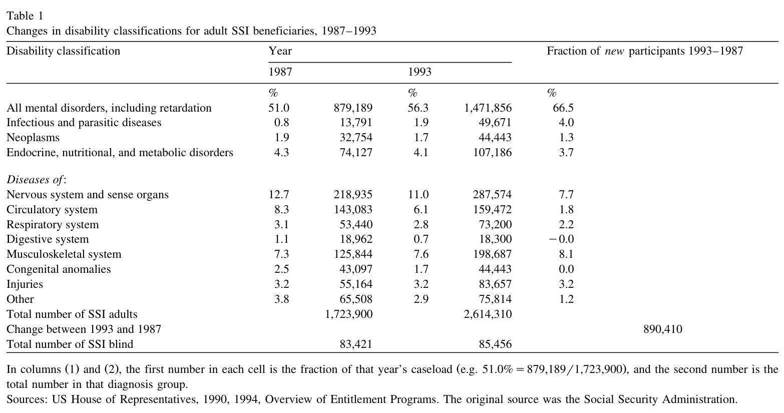
Table 1 presents data originally published by the Social Security Administration on the disability classifications of SSI beneficiaries. These tabulations span the period I analyze, the years 1987 and 1993, and restrict attention to adults aged 18 to 64. During this period, those classified with mental disorders rose by more than five percentage points, from 51.0 to 56.3%. Although the change in the proportion who are mentally disabled may seem modest, the third column shows that two-thirds of the new participants had mental disorders. In contrast, most other disability categories grew far less. In total, the disabled SSI caseload grew by 51%. In contrast, the last row shows that the blind SSI caseload grew by 2.4%.
Although it is more difficult to prove that the health status of the blind was not changing, illustrating what was happening to the blind and disabled SSI caseloads is possible. This is important, because if the caseload growth for the blind was highly correlated with that of the disabled, it may suggest that omitted SSI eligibility represented a more general phenomenon, such as a change in social mores or an easing of the burden to get onto welfare. In either scenario, we might expect the marginal blind SSI participant to be very different from the average blind participant, including his health.
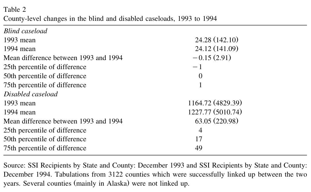
Table 2 presents county-level tabulations of administrative statistics from December 1993 and December 1994.14 Throughout the period, including these two years, the definition of blindness remained constant: vision in the better eye of 20/200 or worse with the use of a corrective lens. As the variable means illustrate, the number of SSI blind remained nearly constant, falling from 24.28 blind per county in 1993 to 24.12 blind in 1994. Thirty-eight percent of the counties (1187 of 3122) had the same number of blind in 1994 as 1993, while another 1013 had a difference of plus or minus one. In contrast, the number of disabled adults in the average county jumped up 5%, from 1164 persons to 1227 persons.
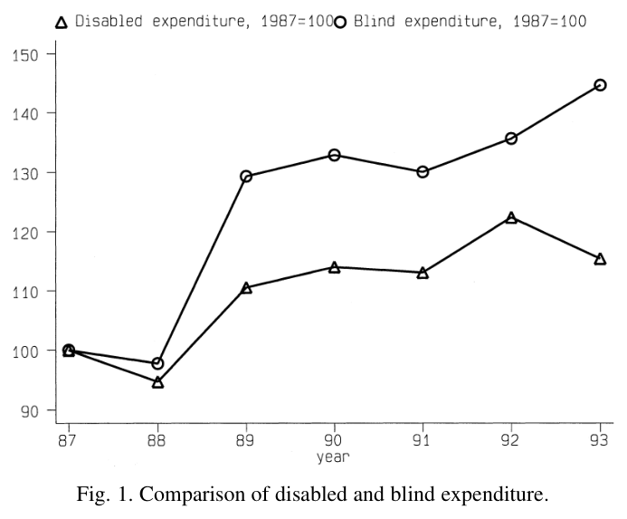
Another implication is that the blind average Medicaid expenditure should grow faster than the disabled average Medicaid expenditure (because the new disabled beneficiaries are healthier). This is illustrated in Fig. 1, where the initial values for average Medicaid expenditure in 1987 are equal to 100, and the subsequent years show the real expenditure relative to the 1987 baseline. The expenditure path of the blind, shown with circles, increased more rapidly than that of the disabled, shown with triangles. By 1993, blind expenditure was 1.45 times its 1987 value, whereas disabled expenditure was 1.15 times the baseline. Expenditure for both groups generally trended upward, of course, because other changes such as physician reimbursement made Medicaid more valuable.
### Table 1. Changes in disability classifications for adult SSI beneficiaries, 1987–1993
Table 1. Changes in disability classifications for adult SSI beneficiaries, 1987–1993 — source page 8. Open full-resolution image · Read source PDF page
In columns (1) and (2), the first number in each cell is the fraction of that year’s caseload (e.g. 51.0% = 879,189/1,723,900), and the second number is the total number in that diagnosis group.
Sources: US House of Representatives, 1990, 1994, Overview of Entitlement Programs. The original source was the Social Security Administration.
### Table 2. County-level changes in the blind and disabled caseloads, 1993 to 1994
Table 2. County-level changes in the blind and disabled caseloads, 1993 to 1994 — source page 9. Open full-resolution image · Read source PDF page
**Notes:** Source: SSI Recipients by State and County: December 1993 and SSI Recipients by State and County: December 1994. Tabulations from 3122 counties which were successfully linked up between the two years. Several counties (mainly in Alaska) were not linked up.
### Figure 1. Comparison of disabled and blind expenditure
Figure 1. Comparison of disabled and blind expenditure — source page 9. Open full-resolution image · Read source PDF page
A final issue concerns the explanatory power of the first-stage regression. The instrumental variables strategy assumes higher spending on the blind shows that the underlying generosity of the program for the disabled is higher. Still, this is not necessarily the case, as the blind and the disabled may use a very different set of providers. Although the t-statistic in the first-stage shows that blind expenditure translates into higher disabled expenditure, showing that payments for the blind are picking up variation in program generosity that might spill over to the disabled is instructive. To illustrate this, I obtained a geographic cost index for 1993, and calculated the correlation between physician practice expenses and blind average Medicaid expenditure.15 This correlation was 0.298, showing those states with higher blind expenditure had higher physician expenses.16
### 2.4. Prior studies of Medicaid and welfare participation
While Medicaid was introduced thirty years ago and program costs have been soaring, only recently has it garnered much academic interest. One reason Medicaid’s effect on SSI participation has been ignored is because the behavioral elasticities of the blind, elderly, and disabled were believed to be extremely small.
In addition, estimating Medicaid’s impact on welfare participation is complicated by the high correlation between eligibility for Medicaid and cash benefits for the disabled. While few examinations of Medicaid and SSI exist, several studies have looked at the impact of Medicaid on AFDC participation and work effort. The earlier studies found that Medicaid had a surprisingly small effect on the welfare and work choices for female heads, but more recent work has found larger effects.
Blank (1989) uses cross-sectional variation in average Medicaid expenditure, which varies tremendously across states, to examine AFDC participation.17 Using data from the 1980 National Medical Care Utilization and Expenditure Study (NMCUES), she finds that health problems significantly increase AFDC participation, but that program rules do not. The insignificant effect of the Medically Needy (MN) program is not surprising because eight of the thirty MN states in her sample had an income eligibility level below the maximum AFDC payment level.
What is surprising is the robustness of the finding that the state-specific Medicaid insurance value did not affect AFDC participation.
Moffitt and Wolfe (1992) construct an individual-specific valuation of health insurance to surmount Medicaid’s collinearity with AFDC eligibility. They note that a Medicaid variable constructed from a state-specific average may badly measure Medicaid’s value for any particular family. Linking the 1984 Survey of Income and Program Participation (SIPP) and 1980 NMCUES, they construct a ‘heterogeneity’ index for Medicaid’s value based on different health characteristics of the woman and her family. This index yields enormous variation in Medicaid’s value. Using this variation, they find sizable effects of Medicaid on labor market outcomes.
I examined expansions in Medicaid eligibility targeted toward young children from 1988 to 1991 (Yelowitz, 1995). These expansions linked Medicaid eligibility to the federal poverty line rather than a state’s AFDC income eligibility limit, thus offering an incentive to leave welfare. I found that these reforms significantly decreased AFDC participation and increased labor force participation. Among female headed households, the effects were largest for previously married women, but were negligible for never-married women.
Very little evidence exists on the interaction of Medicaid and SSI. Rupp and Stapleton (1995) find no association between Medicaid and SSI applications (which differs from participation), but their OLS specification does not account for problems of omitted variables bias and measurement error. I examined recent changes in the Medicaid program on the SSI participation for a different group, senior citizens (Yelowitz, 1996). By using the implementation of a buy-in program for Medicare in the 1980s (which offered a substitute for the cost-sharing provisions of Medicaid), I found significant interactions: Medicaid had a bigger impact on exits from SSI for the elderly than it had on exits from AFDC for female heads.
## 3. Theoretical considerations
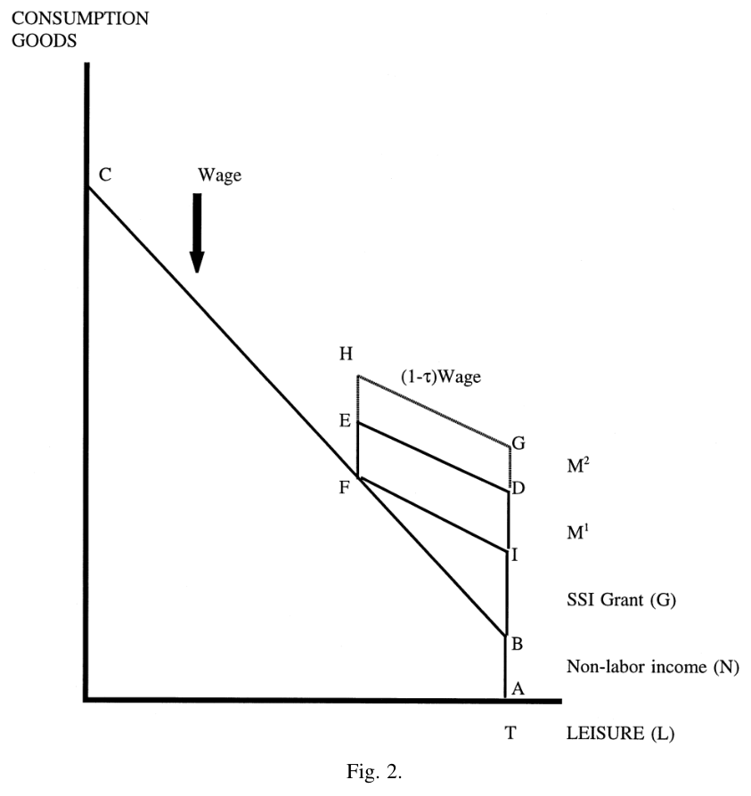
This section briefly outlines several ways that Medicaid’s value influences SSI participation. The individual maximizes a utility function, , which is a function of consumption goods () and leisure (). The price of consumption goods () is normalized to US$1 per unit, while the price of leisure is simply the wage rate (). He is given a time endowment () which he can allocate between work and leisure. He may also receive nonlabor income (), for instance from the earnings of his spouse. Therefore, his full budget constraint is initially defined as:
In Fig. 2, this is represented as the segment ABC. Given this budget constraint, the consumer maximizes his utility.
By introducing the SSI system into the model, the government changes the budget constraint. The program offers a grant (), which was US$652 per month for a married couple in 1993, and reduces this grant for earning income in the labor market. This reduction, known as the ‘benefit reduction rate’ (), is 50% on earned income. Therefore, the net wage falls to along the initial part of the budget constraint. The budget constraint with SSI cash benefits is characterized by the segment AIFC.
The final institutional feature is Medicaid. Broadly speaking, Medicaid is received when the individual is on SSI, and is entirely lost after leaving SSI. This discrete drop in benefits is known as the ‘Medicaid notch’—the design of the program creates part of the budget constraint where no utility maximizing person should choose to be.
Variation in the value of Medicaid changes the budget constraint. Consider an individual who lives in a state where Medicaid is valued at some small amount, —this can be thought of as the dollars the family would have to spend on medical expenses without insurance. His budget constraint now is represented by ADEFC in Fig. 2. Consider a second individual who lives in a different state that has the same SSI grant but a more generous Medicaid program, so that the value is + . In this state, the budget constraint is represented by AGHFC.
### Figure 2. Fig. 2.
Figure 2. Fig. 2. — source page 12. Open full-resolution image · Read source PDF page
By increasing Medicaid’s value from to , SSI participation could increase for two reasons. First, a person who was initially found somewhere along the segment FC (i.e., initially ineligible) may now find that he receives higher utility on segment GH, and therefore cuts back on his hours of work. Second, some who were eligible and initially on segment BF (i.e., nonparticipating eligibles) now find Medicaid’s value high enough that it outweighs the stigma cost of welfare.18 Two other assumptions deserve mention. First, the model assumes that the individual does not have access to private health insurance. Clearly, the importance of Medicaid and its effect on SSI participation should be much more important for individuals without other health insurance options such as employer coverage. If the scope of services from Medicaid differs from the private package, however, Medicaid may still have some effect on those with ‘‘private coverage’’.
Second, the model does not account for the effects of health status on labor supply and SSI participation.19 Poor health has at least three different effects on the budget constraint. It lowers the wage that the individual can receive in the labor market either by limiting the type of job and hours of work he can take, or by lowering his productivity. Poor health also changes preferences toward work and leisure: at any bundle, the marginal rate of substitution rises with poor health.
Finally, poor health increases the value of Medicaid—since expected utilization is higher, the benefits are worth more than before. Unless accurate proxies for the individual’s health status can be found, models relying on variation in Medicaid’s value generated by health status may mistakenly attribute changes in preferences, productivity, and wages to Medicaid.
## 4. Descriptive analysis
I use the 1988–94 CPS March annual demographic file, which provides retrospective information on family income, health insurance coverage, and program participation from 1987 to 1993 for the noninstitutionalized population. Because only a small fraction of the adult population participates in SSI-disabled, a large data set is essential to observe trends. Therefore, the CPS is perhaps a more useful household data set than others.
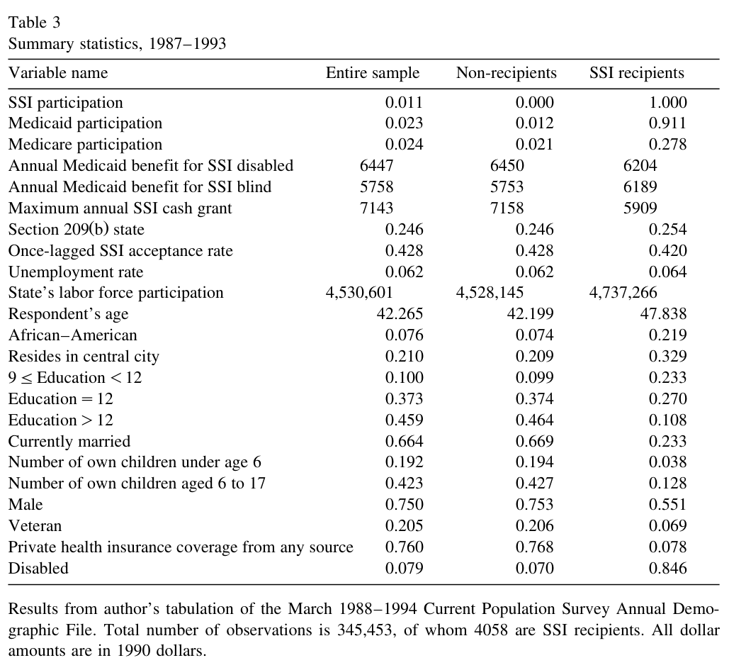
I use about one-third of the roughly 1.05 million observations contained in the 1988–1994 CPS files. The most important exclusions are the following: being over the age of 64, being under the age of 18, living in Arizona, having imputed information on SSI or Medicaid receipt, having an imputed spouse number, being a woman under the age of 45, being a race other than African–American or white, living in a single parent household, or having more related children than own children in a family.20 Table 3 presents summary statistics for the variables used in the analysis, for the entire population, SSI nonrecipients, and SSI recipients. Since only 4058 of the 345,453 observations are SSI recipients, the means of demographic variables for the nonrecipients closely match those of the entire population. In column (1), SSI participation is 1.17%, while Medicaid participation is nearly double that number, 2.30%. Even with the exclusion of single parent households, some families may have access to Medicaid from sources other than SSI-disabled.
Part of the gap between the two participation rates could be the result of the existing Medically Needy and General Assistance programs. Moving to column (3), 91% of SSI recipients also report Medicaid coverage. There are at least two reasons why Medicaid participation may not be complete for SSI recipients. First, the survey respondent might report Medicaid receipt only if he went to the hospital or physician. Second, because some states require a second application for Medicaid, the respondent may not apply for benefits until he becomes sick. This table also shows Medicare participation averages 27.8% for SSI recipients and 2.1% for nonrecipients. Since an SSI recipient is much more likely to participate in the disability insurance (DI) program than a nonrecipient, a prolonged
SSI spell can result in Medicare coverage. A nonrecipient can also qualify for DI and by that qualify for Medicare.
The next five rows in Table 3 illustrate state-level policy variables characterizing the Medicaid and SSI programs.21 The unit of observation remains the individual; thus, the variable means implicitly give more weight to observations from larger states. In column (1), the average Medicaid expenditure per disabled SSI recipient is US$700 higher than for a blind SSI recipient. The maximum annual SSI grant (including the state supplements) exceeds average Medicaid expenditure by US$800. There are large differences in the benefit levels between SSI recipients and nonrecipients: columns (2) and (3) show that nonrecipients live in states with modestly higher average Medicaid expenditures and much higher SSI grants. On the surface, these differences would suggest that higher benefits reduce participation. Other omitted factors, such as attitudes toward welfare participation, vary across states and are surely correlated with benefit levels, however. Around one-quarter of the sample live in a 209(b) state, meaning that the SSI participant must file another application to receive Medicaid. Finally, the once-lagged SSI acceptance-to-application rate is 42%. The lagged acceptance rate falls steadily until 1989 (when it is 39%) and then trends upward afterwards, reaching a high of 48% in 1993.
### Table 3. Summary statistics, 1987-1993
Table 3. Summary statistics, 1987-1993 — source page 15. Open full-resolution image · Read source PDF page
**Notes:** Author's tabulation of the March 1988-1994 Current Population Survey Annual Demographic File. There are 345,453 observations, of whom 4,058 are SSI recipients. Dollar amounts are in 1990 dollars.
### Figure 3. Trends in SSI and Medicaid participation
Figure 3. Trends in SSI and Medicaid participation — source page 16. Open full-resolution image · Read source PDF page
The next two rows show the means of economic variables included in the model. SSI recipients live in states with higher unemployment and large labor force pools. A study by Stapleton et al. (1995) found that changes in the unemployment rate accounted for 10% of the growth in SSI applications from 1988 to 1992.
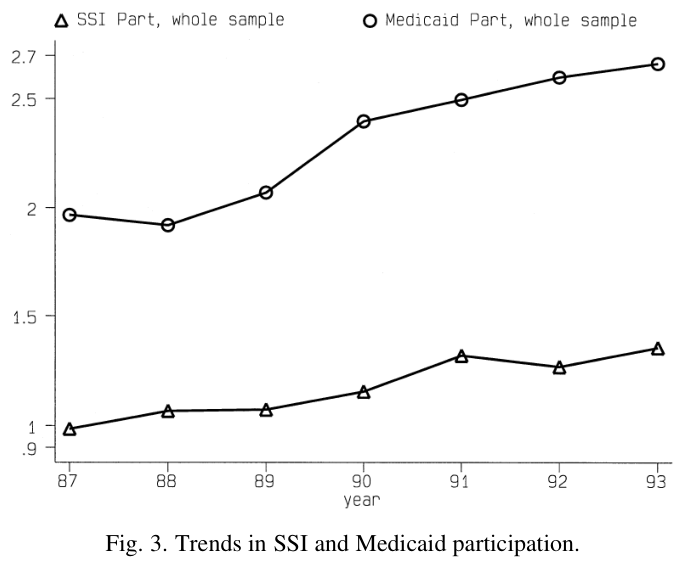
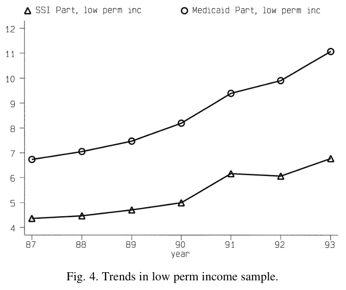
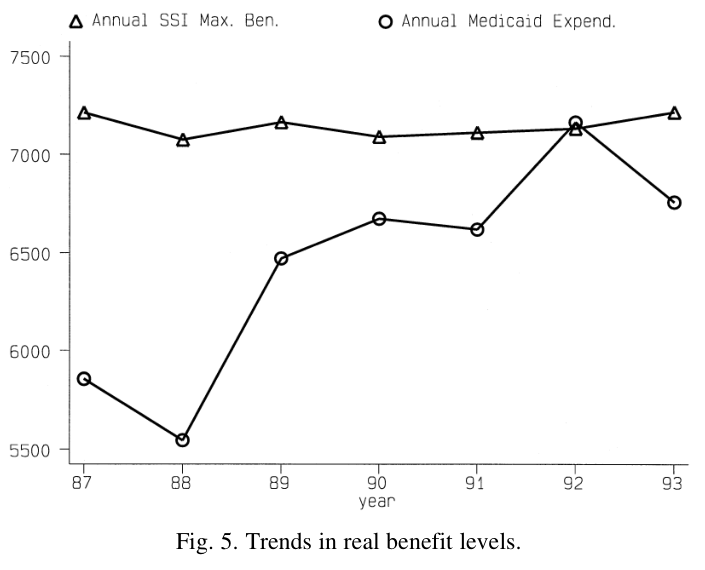
Finally, Table 3 displays several demographic characteristics included in the regression analysis. On average, SSI recipients are five years older than nonrecipients. Participants are much more likely to be African–American. In addition, SSI recipients are far less educated: 38% did not even enter high school, and another 23% did not complete high school. In contrast, only 16% of nonrecipients did not receive at least a high school diploma. SSI recipients are less likely to be married, be male, have children, or be a veteran. There are also stark differences in the take-up (and presumably availability) of private insurance coverage and in the extent of self-reported disability. Less than 8% of SSI recipients had private coverage, compared with 77% of nonrecipients. An overwhelming fraction of SSI participants report disability, while few nonparticipants report this.22 Fig. 3 and Fig. 4 break out the trends in SSI participation from 1987 to 1993, for the entire sample and a group with low permanent income, those aged forty and over who are high school dropouts. For the entire sample, the SSI participation rate rose steadily, from 0.98% in 1987 to 1.35% in 1993. Participation rose more dramatically for those with low permanent income, rising from 4.36% to 6.78%. The figures also show how Medicaid participation evolved over time. For both the full sample and the low permanent income sample, Medicaid participation exceeded SSI participation. It rose from 1.96% to 2.66% in the full sample, and by 4.35 percentage points for the low permanent income sample, from 6.73% to 11.08%. Fig. 5 presents trends in SSI benefits and average Medicaid expenditure.23 The potential SSI benefit is computed from the CPS, based on the respondent’s state of residence, year, and marital status. Clearly, two different patterns emerge here. Real SSI cash benefits were unchanged. This is expected since the federal benefit level is indexed for inflation. Average Medicaid expenditure for the disabled increased by close to US$1000 (or roughly 15% of its 1987 value) in real terms.
### Figure 4. Trends in low permanent income sample
Figure 4. Trends in low permanent income sample — source page 17. Open full-resolution image · Read source PDF page
### Figure 5. Trends in real benefit levels
Figure 5. Trends in real benefit levels — source page 17. Open full-resolution image · Read source PDF page
This rise in average Medicaid expenditure mirrors the rise in overall SSI participation rates; thus, this is at least suggestive that a link exists between average Medicaid expenditure and SSI.
## 5. Regression results
### 5.1. OLS estimates using average Medicaid expenditure of the disabled
For ease of interpretation, I present results from a linear probability model.24 The coefficients from the models below therefore may be interpreted as percentage point changes. The basic equation is given by:
In this equation, i subscripts individuals, j subscripts states and t subscripts time. The outcome, SSI participation () is a binary variable equal to 1 if the respondent participated in the program in the previous year.25 Increases in two key policy variables, average Medicaid expenditure () and the SSI grant (), are expected to increase SSI participation. I also include two other state-specific variables that proxy for outreach effort or encouragement to enroll in Medicaid. These variables are whether the respondent lived in a Section 209(b) state, and the once-lagged SSI acceptance rate. Several states changed 209(b) status during the period, which allows the coefficient to be identified even in models including state-fixed effects. The sign of the coefficient is likely to be negative—living in a state with extra application procedures for Medicaid may increase transaction costs, and 209(b) states typically have more restrictive eligibility requirements for Medicaid than SSI. The lagged SSI acceptance rate measures the stringency that a state uses in evaluating disability. The business cycle variables () include the annual unemployment rate in the state and the number participating in the labor force.26 The vector contains several individual level variables that may also influence SSI participation, including the respondent’s age and its square, race, residence in a central city, education, marital status, number of children present, gender, and veteran status.27 In addition, I amend this basic specification to allow for nationally uniform, time-varying shocks to SSI participation through the inclusion of time dummies, and time-invariant, state-specific shocks to SSI participation through the inclusion of state dummies.28 The coefficients , , , , , , and are to be estimated, and is an error term. Finally, the standard errors in both the OLS and TSLS specifications are corrected for group correlations within state-year cell, since the policy variables vary at the state-year level, but the unit of observation is the individual. Moulton (1986) explains that the standard errors can be dramatically understated without correcting for these correlations.
By including time fixed effects (), the regression framework accounts for other factors that may lead to an increase in SSI participation. I can control for the effects of the business cycle (at the national level) with the time dummies. If changing economic conditions are correlated with average Medicaid expenditure, the results will be biased by not accounting for this omitted variable. Time dummies also control for three other sources of SSI growth. First, SSI spell lengths may have increased in duration because SSA was doing fewer disability reviews. Second, some medical breakthroughs may have allowed disabled people to live longer than they otherwise would have. Third, SSA conducted outreach efforts, which may have attracted new recipients.
Several omitted variables, which vary by state, could bias the results. Including state-fixed effects () in the regression addresses these concerns. For example, the availability of Medicaid coverage varies across states and this could affect SSI participation. A poor adult may be able to receive health insurance coverage through the Medically Needy (MN) or General Assistance (GA) programs. These programs may be correlated with average Medicaid expenditure and affect SSI participation without the inclusion of state-fixed effects.
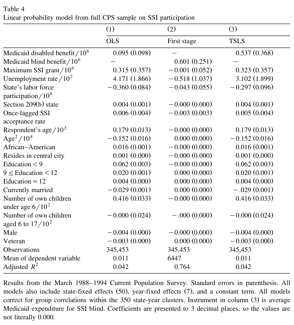
The result in the first column of Table 4 shows that the OLS estimate of b is statistically insignificant and economically unimportant. The point estimate implies that increasing Medicaid by US$1000 leads to an increase in SSI participation of 0.0095 percentage points. Since Fig. 5 illustrates that average Medicaid expenditure for the entire sample rose in real terms from US$5855 in 1987 to US$6759 in 1993, this coefficient estimate implies that increased average Medicaid expenditure raised the probability of SSI participation by 0.0085 percentage points. SSI participation for the whole sample increased from 0.98 to 1.35% (or 0.370 percentage points); thus, the OLS estimate implies that rising health care costs can explain around 2.3% of the rise in SSI participation.
### Table 4. Linear probability model from full CPS sample on SSI participation
Table 4. Linear probability model from full CPS sample on SSI participation — source page 20. Open full-resolution image · Read source PDF page
**Notes:** Results from the March 1988-1994 Current Population Survey. Standard errors are in parentheses. All models also include state fixed effects (50), year fixed effects (7), and a constant. All models correct for group correlations within 350 state-year clusters. The instrument in column (3) is average Medicaid expenditure for SSI blind. Coefficients are shown to three decimal places, so values displayed as 0.000 are not literally zero.
Cash benefits do not seem to affect SSI participation. Increasing the SSI cash benefit appears to lower SSI participation, but the coefficient is not significant. The table also shows the effect of a third policy variable: residence in a Section 209(b) state—one that requires a second, separate application for Medicaid.
Contrary to expectations, living in a 209(b) state raises the probability of participating in SSI. One caution in interpreting this coefficient, however, concerns legislative endogeneity. The states that switched to 209(b) status may have done so because the SSI rolls were increasing. The lagged SSI acceptance rate does not seem to affect participation either.
The business cycle variables enter in the appropriate direction. In the OLS specification, increases in the unemployment rate raise SSI participation and increases in the labor force pool lower it. The coefficient on the unemployment rate implies that a 2.3 percentage point increase in the unemployment rate has the same effect on SSI participation as a US$1000 increase in Medicaid. Similarly, a contraction in the labor force of 26,480 persons has the same effect on participation.
Education and family structure play important roles in SSI participation. Relative to those with a college degree, individuals with less than nine years of education are 6.2 percentage points more likely to participate in SSI, while those with less than 12 years are 2.0 percentage points more likely to participate. In addition, those who only completed high school are more likely to participate in the SSI disabled program than those who entered college, but the economic impact is not as dramatic as for the other educational groups. Being married lowers SSI participation by 2.9 percentage points, while the presence of another young child increases the probability of participation.
The signs of the other demographic and location-specific characteristics enter the SSI participation equation largely as expected. SSI participation increases with age, but at a decreasing rate. The point estimates show that SSI participation increases all the way until age 64. Since many physical disabilities may not occur until later ages, this finding is plausible. Relative to whites, being African-American raises the probability of SSI participation by 1.6 percentage points.
Living in a central city raises SSI participation. This may occur for two reasons. First, those in central cities may have greater access to welfare and Social Security offices or health care facilities, which lowers the transaction costs of SSI participation, and raises the value of Medicaid, respectively. Second, if living in a central city means that the individual has better information about the programs, he would be more likely to participate. Finally, being male or being a veteran significantly lowers SSI participation.
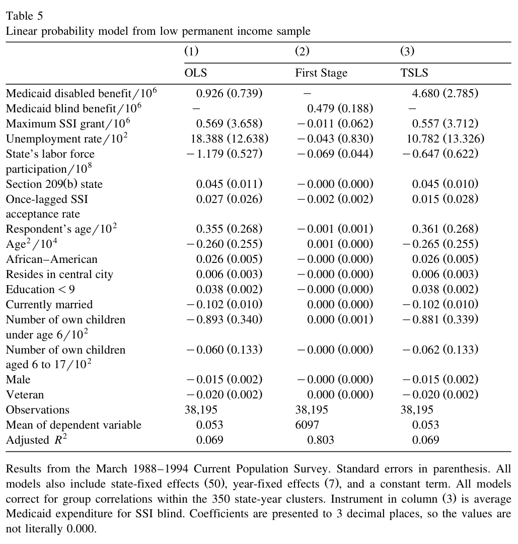
### Table 5. Linear probability model from low permanent income sample
Table 5. Linear probability model from low permanent income sample — source page 22. Open full-resolution image · Read source PDF page
models also include state-fixed effects (50), year-fixed effects (7), and a constant term. All models correct for group correlations within the 350 state-year clusters. Instrument in column (3) is average Medicaid expenditure for SSI blind. Coefficients are presented to 3 decimal places, so the values are not literally 0.000.
Table 5 presents analogous results for the low permanent income sample, high school dropouts aged 40 to 64. There are two separate motivations for examining this group. First, SSI participation is a somewhat rare outcome for the full sample and it is useful to show that the results are similar for a sample where it is more common. Second, it is expected that this group should have larger responses to Medicaid policy than the full sample, because alternative sources of health insurance are less common. As column (1) of this table shows, this group does respond more to changes in Medicaid’s value. For a US$1000 increase in Medicaid’s value, SSI participation rises by 0.0926 percentage points, an order of magnitude larger than for the full sample. Medicaid explains a larger fraction of the growth. The increase of US$1052 in Medicaid’s value explains 4% (= 1.052 × 0.000926 / 0.0241) of the growth in SSI participation.
### 5.2. Instrumental variable estimates
The prior estimates used variation in disabled average Medicaid expenditure. These may be biased if changes in the underlying health of the SSI population affected both Medicaid’s value and SSI participation. If the eligibility criteria for disability become less strict, for example, so that people who were previously found ineligible are now deemed eligible for SSI, then the former estimates of β₁ would be too small. In the Supreme Court’s _Sullivan v. Zebley_ decision, such a reevaluation occurred for children, and this may have had spillovers into the adult population.29 In addition, if states attempted to shift their General Assistance and Medically Needy beneficiaries onto the SSI rolls, and if these groups happened to be healthier, the OLS results would be biased. In this case, the marginal disabled SSI recipient will likely incur less health care expenditure than the average recipient, so that average expenditure falls while SSI participation increases. This would lead to a spurious negative correlation (which in turn biases the coefficient downward).
To correct for this bias, I instrument for average Medicaid expenditure of the disabled in each state-year cell with the corresponding average expenditure of the blind SSI recipients. This variable reflects different aspects of the state’s Medicaid program that influence its value, such as variation in health care prices, access to care, and scope of services. Since the criteria to qualify is more objective, then this instrument is unlikely to be correlated with changing definitions of disability.
Returning to Table 4, the middle column presents the result of the first stage. The instrument is highly correlated with the average Medicaid expenditure of the disabled: the coefficient on expenditure for the blind has a _t_ -statistic of 2.4 and the _R_2 of the first stage regression is 0.76.30 By instrumenting, the coefficient estimate in the third column of Table 4 increases, consistent with changing the budget constraint in Fig. 2. Increasing average Medicaid expenditure by US$1000 is now associated with an increase in the probability of SSI participation by 0.0537 percentage points. Again, taking the rise in average Medicaid expenditure from Fig. 5, this estimate implies that rising health care costs raised the probability of participation by 0.0485 percentage points. Since the total increase in SSI participation was 0.370 percentage points, then rising healthcare costs explain approximately 13% of the rise in SSI participation. The point estimates on the other individual level explanatory variables are similar to the OLS specification. Some other variables that vary at the state–year level are less precisely estimated than in the OLS specification. In particular, the coefficient on the unemployment rate and the state’s labor force pool fall by one quarter.
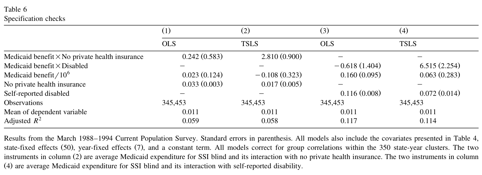
### Table 6. Specification checks
Table 6. Specification checks — source page 24. Open full-resolution image · Read source PDF page
state-fixed effects (50), year-fixed effects (7), and a constant term. All models correct for group correlations within the 350 state-year clusters. The two instruments in column (2) are average Medicaid expenditure for SSI blind and its interaction with no private health insurance. The two instruments in column (4) are average Medicaid expenditure for SSI blind and its interaction with self-reported disability.
The conclusions for the low-permanent income sample in Table 5 are stronger than for the full sample. In the first stage, the coefficient on expenditure for the blind has a t-statistic of 2.5 and the R2 of the first stage regression is 0.80. The results from TSLS tell the same basic story, and the coefficient estimate on average Medicaid expenditure is statistically significant at the 90% level. The TSLS estimates in column (3) are much larger than the OLS estimates, and Medicaid explains approximately 20% of the growth in SSI participation for this group.
Finally, I did two specification checks, presented in Table 6. First, I interacted an indicator variable for ‘No Private Insurance Coverage’ with average Medicaid expenditure, and included the main effects (that is, a dummy for no private coverage enter alone and the Medicaid variable entered alone). The intuition behind this interaction is that Medicaid’s rising value should matter most for those without private coverage, and should not affect those with coverage. The model now includes two endogenous variables: the interaction of insurance coverage with the Medicaid benefit, and the Medicaid benefit. These are instrumented with the interaction of insurance coverage and the blind Medicaid benefit, and the blind Medicaid benefit entered by itself. Column (2) presents the results of the TSLS estimation.
The results show that average Medicaid expenditure has a strong, positive effect on SSI participation for those without other sources of coverage, and does not affect those with other sources of coverage.
Second, I use the one-health status measure asked in the March CPS: ‘Does the respondent have a health problem or a disability which prevents him or her from working or which limits the kind or amount of work’. Similar to the reasoning for ‘No Private Health Insurance Coverage’, the interaction of disability and average Medicaid expenditure should be positive. As column (4) shows, average Medicaid expenditure has a strong effect on the disabled, and no effect on the nondisabled.
## 6. Conclusions and extensions
This paper finds that rising health insurance costs are an important reason for participation in the SSI-disabled program. By using a large, nationally representative household data set, I find that 13 to 20% of the rise in SSI participation may be due to increases in the value of Medicaid.
I show that ordinary least squares produces a badly biased estimate, since the health status of the disabled population is changing. The estimates using instrumental variables produce a much stronger positive effect of Medicaid on SSI participation. Is it reasonable to assume that the health status of the disabled changed so dramatically while the health status of the SSI blind did not? Knowing the answer to this question is vital for assessing the validity of the instrument.
Although proving that the health of the blind remained constant is difficult, analysis of caseload changes shows that the year-to-year change for blind SSI recipients is extremely small, which makes it likely that the same blind individuals remain on SSI from one year to the next.
Are the estimated effects too large? At this point, considering findings on other Medicaid populations is relevant. In other work, I found significant effects on AFDC participation for female heads and on SSI participation for elderly households (Yelowitz, 1995, 1996). In those studies, the policy changes were different from those in this study, however. The policy changes were for young children and the elderly who are offered Medicaid without the need to apply for AFDC or SSI. In an approach more similar to the current study, Moffitt and Wolfe (1992) value Medicaid and find strong effects on AFDC participation for female heads.
Their findings imply that a 15% increase in the value of Medicaid benefits would increase the AFDC caseload about 2.7%. The findings in this paper show that a similar increase in Medicaid’s value leads to a 13 to 20% increase in SSI participation. It is plausible that health insurance plays a more important role in the economic decision-making of disabled adults than female heads, so the effects appear reasonable.
The findings have several policy implications for program design. If Medicaid is an important determinant of SSI participation, then offering health insurance without the need to participate in SSI may reduce total costs. This could occur because disabled adults may then forego the cash benefits from SSI. The effects on SSI’s total cost are likely to be modest, however. Of the 1.1 million new recipients who joined between 1987 and 1993, roughly 15% (or 165,000) joined because of the rise in Medicaid. The average annual benefit paid to SSI recipients in 1993 was US$4236. This annual benefit surely represents an upper bound on the amount paid to new recipients, because they are in better health and may have some labor market earnings. Assuming this benefit level is correct, US$700 million out of US$16.5 billion spent on cash benefits for the disabled could have been saved if the programs had not been linked, or 4.2% of SSI costs.
On the other hand, some disabled adults who were not previously participating in SSI because of the stigma associated with the program may decide to participate in a Medicaid-only program, which could increase costs. This might already occur through the Medically Needy program, which many states offer, however. Since the MN program typically has lower income limits than SSI and fewer covered services under Medicaid than for categorically needy recipients, it may not offer enough of an incentive for the disabled to leave.
Perhaps the most useful extension of the current study would be to develop a model that includes a broadened look at the effects of health on SSI participation, similar to Wolfe and Hill (1995). This would be important for two reasons. First, by examining a data set with better measures of health, one could test directly the hypothesis that disabled SSI recipients became healthier. Second, by incorporating health directly into the SSI participation equation, it may be possible to see which type of disabled person responds to different government policies concerning extension of Medicaid benefits.
## Acknowledgements
Work on this paper was supported by the Office of the Assistant Secretary for Planning and Evaluation in the US Department of Health and Human Services, the Social Security Administration, and the National Institute on Aging. I am grateful for helpful comments and encouragement from Joshua Angrist, Rebecca Blank, Janet Currie, David Cutler, Leora Friedberg, Jonathan Gruber, Hilary Hoynes, Wei-Yin Hu, Jacob Klerman, Caroline Minter Hoxby, Steven Levitt, Jorn-Steffen Pischke, James Poterba, Douglas Staiger, David Stapleton, Duncan Thomas, Barbara Wolfe, two anonymous referees, editor Joseph Newhouse, and participants at National Bureau of Economic Research and the Social Security Administration. Gloria Chiang provided excellent research assistance. The STATA programs and data used in this study may be obtained from the author.
## Appendix A. Sources
### A.1. Current population survey
An appendix table showing the sample selection criteria is available from the author.
### A.2. Average Medicaid expenditure data
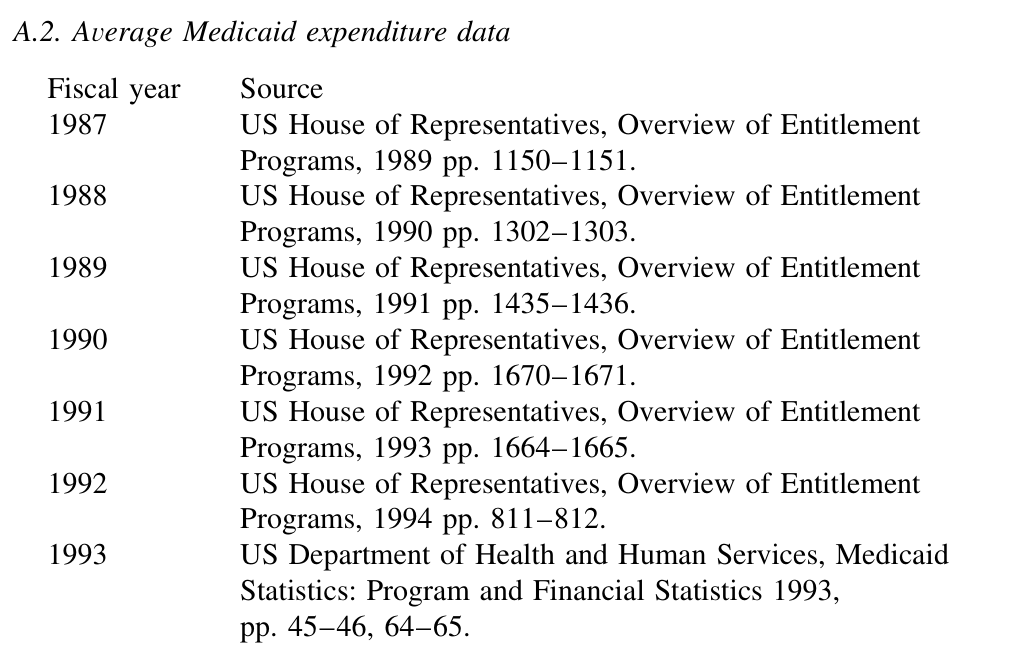
### Appendix table. Average Medicaid expenditure data
Appendix table. Average Medicaid expenditure data — source page 27. Open full-resolution image · Read source PDF page
A.3. SSI benefit data US House of Representatives, Overview of Entitlement Programs, 1991, pp. 741–742. US House of Representatives, Overview of Entitlement Programs, 1993, pp. 824, 829–830. A.4. Unemployment rate and labor force participation Bureau of Labor Statistics. Local Area Unemployment Statistics—Annual Measures of the Unemployment Rate and the Total Civilian Labor Force. Available by World Wide Web at http://stats.bls.gov:80/lauhome.htm.
A.5. Price indices for general inflation and medical prices Council of Economic Advisers, 1995; Economic Report of the President. Table B-61, p. 344. A.6. Medicaid 209(b) status US House of Representatives, Overview of Entitlement Programs, 1988 p. 798.
US House of Representatives, Overview of Entitlement Programs, 1989 p. 1129. US House of Representatives, Overview of Entitlement Programs, 1990 p. 1278. US House of Representatives, Overview of Entitlement Programs, 1991 p. 1406. US House of Representatives, Overview of Entitlement Programs, 1992 p. 1642.
US House of Representatives, Overview of Entitlement Programs, 1993 p. 1635. A.7. SSI acceptance rates Lewin-VHI, 1995. Public use data file on the Social Security Administration’s disability programs [unpublished manuscript].
## References
Adams, E.K., 1994. Effect of increased medicaid fees on physician participation and enrollee service utilization in Tennessee, 1985–1988. Inquiry 31 (2), 173–187.
Angrist, J., 1991. Instrumental variables estimation of average treatment effects in econometrics and epidemiology, technical working paper 115. Natl. Bureau of Economic Res., Cambridge, MA.
Angrist, J., Krueger, A., 1991. Does compulsory school attendance affect schooling and earnings?. Q. J. Economics 106 (4), 979–1014.
Blank, R., 1989. The effect of medical need and medicaid on AFDC participation. J. Human Resources 24 (1), 54–87.
Bound, J., Jaeger, D., Baker, R., 1995. Problems with instrumental variables estimation when the correlation between the instruments and the endogenous explanatory variable is weak. J. Am. Statistical Association 90 (430), 443–450.
Congressional Research Service, 1988. Costs and effects of extending health insurance coverage. US Government Printing Office, Washington, DC.
Council of Economic Advisers, 1995. Economic report of the President. US Government Printing Office, Washington, DC.
Currie, J., Gruber, J., Fischer, M., 1995. Physician payments and infant mortality: evidence from Medicaid fee policy. Am. Economic Rev. 85 (2), 106–111.
Decker, S., 1993. The effect of physician reimbursement levels on the primary care of medicaid patients. New York Univ., Wagner School of Public Service, unpublished manuscript.
Gruber, J., Madrian, B., 1994. Health insurance and job mobility: the effects of public policy on job-lock. Industrial and Labor Relations Rev. 48 (1), 86–102.
Holahan, J., Rowland, D., Feder, J., Heslam, D., 1993. Explaining the recent growth in Medicaid spending. Health Affairs 12 (3), 177–193.
Kubik, J., 1996. Is disability endogenous? The SSI disability program and the health of children. Massachusetts Inst. of Technol., unpublished manuscript.
Lahiri, K., Vaughan, D., Wixon, B., 1995. Modeling SSA’s sequential disability determination process using matched SIPP data. Social Security Bull. 58 (4), 3–42.
Moffitt, R., 1983. An economic model of welfare stigma. Am. Economic Rev. 73 (5), 1023–1035.
Moffitt, R., 1993. The effect of work and training programs on entry and exit from the welfare caseload, discussion paper 1025-93. Inst. for Res. on Poverty, Madison, WI.
Moffitt, R., Wolfe, B., 1992. The effect of the medicaid program on welfare participation and labor supply. Rev. Economics and Statistics 74 (4), 615–626.
Moffitt, R., Ribar, D., Wilhelm, M., 1996. The decline of welfare benefits in the US: the role of wage inequality. Johns Hopkins Univ., unpublished manuscript.
Moulton, B., 1986. Random group effects and the precision of regression estimates. J. Econometrics 32 (3), 385–397.
Rones, P., 1981. Can the current population survey be used to identify the disabled?. Monthly Labor Rev. 104 (6), 37–38.
Rupp, K., Stapleton, D., 1995. Determinants of the growth in the Social Security Administration’s disability programs—an overview. Social Security Bull. 58 (4), 43–70.
Social Security Administration, 1995. Annual Statistical Supplement.
Stapleton, D., Coleman, K., Dietrich, K., 1995, Demographic and economic determinants of recent application and award growth for SSA’s disability programs. Unpublished manuscript, Lewin-VHI.
US General Accounting Office, 1995. Social security: Federal disability programs face major issues, GAO/T-HEHS-95-97. Statement of Jane Ross, Director, Income Security Issues Health Education and Human Services Division.
US House of Representatives, 1993, Medicaid source book: Background data and analysis (A 1993 update). Government Printing Office, Washington, DC. US House of Representatives, various editions, Overview of entitlement programs: background materials and data on programs within the jurisdiction of the committee on ways and means.
Government Printing Office, Washington, DC.
Winkler, A., 1991. The incentive effects of medicaid on women’s labor supply. J. Human Resources 26 (2), 308–337.
Wolfe, B., 1980. How the disabled fare in the labor market. Monthly Labor Rev. 103 (9), 48–52.
Wolfe, B., 1981. The CPS, work, and disability: a reply. Monthly Labor Rev. 104 (6), 38–39.
Wolfe, B., Hill, S., 1995. The effect of health on the work effort of single mothers. J. Human Resources 30 (1), 42–62.
Yelowitz, A., 1995. The medicaid notch, labor supply and welfare participation: Evidence from eligibility expansions. Q. J. Economics 110 (4), 909–939.
Yelowitz, A., 1996. Using the qualified Medicare buy-in program to estimate the effect of Medicaid on the SSI participation of the elderly, discussion paper 1102-96. Inst. for Res. on Poverty, Madison, WI.
**23.** These are deflated using the CPI-U for the SSI benefit level and the medical services CPI for Medicaid.
**29.** The Supreme Court ruled that disability standards for children may not be narrower than those applied to adults. As a result, eligibility criteria for children are based on a child’s developmental delay and limitations on the child’s ability to engage in age-appropriate activities of daily living. This has increased the number of children classified as disabled. Prior to 1990, the same disability criteria that applied to adults were also applied to children.
**30.** Bound et al. (1995) explain that in finite samples, instrumental variables estimates are biased in the same direction as OLS estimates, and the magnitude of the bias of the instrumental variables estimates approaches that of OLS estimates as the between the instruments and the potentially endogenous explanatory variable approaches zero.
## Additional printed notes
**1.** The numbers in this paragraph were computed from information in Social Security Administration (1995).
**2.** Kubik (1996) provides evidence on the SSI caseloads of children.
**3.** These difficulties in defining disability are well known. See Wolfe (1980, 1981) and Rones (1981) for early discussions.
**4.** To illustrate, the Social Security Administration conducted several outreach activities for SSI. If these outreach programs attracted relatively healthy new recipients, then the average health status may have improved. See US House of Representatives (1993), Overview of Entitlement Programs, for a discussion of these activities.
**5.** An analogy with the returns-to-education literature helps motivate the instrumental variables approach used in this study. When estimating a wage equation, the key source of bias is that omitted ability is likely correlated with educational attainment, and most measures of ‘ability’ that one could include are unlikely to completely remove this correlation. By instrumenting, however, one can derive a consistent estimate of the education parameter. See Angrist and Krueger (1991) for a recent example.
**6.** US House of Representatives (1993), Overview of Entitlement Programs.
**7.** The discussion of the disability determination process draws upon Lahiri et al. (1995).
**8.** Thus, the Section 1619 provisions which are intended to help recipients leave SSI may actually encourage SSI participation through an ‘entry effect’. Moffitt (1993) discusses these ‘entry’ and ‘exit’ effects in the context of the AFDC program with work training requirements.
**9.** Required coverage includes inpatient and outpatient hospital services, rural health clinic services, federally qualified health center services, laboratory and X-ray services, nursing facility services for individuals under age 21, family planning services, physicians’ services, home health services for any individual entitled to nursing facility care, nurse–midwife services, and services of certified nurse practitioners.
**10.** The expenditure numbers on the disabled throughout will include Medicaid spending in intermediate care facilities and skilled nursing homes. It is important to include this component because access to these facilities is, indeed, a part of Medicaid’s value. While only a small portion of the population will become institutionalized, it is also true that only a small portion will use any particular Medicaid service.
**11.** See Holahan et al. (1993) for a detailed explanation.
**12.** See the discussion in Adams (1994) for a more complete review of the literature.
**13.** The assumption that underlies the analysis is the cost of services, not quantity, determines Medicaid’s value. This assumption is made because the alternative is to pay for medical care out-of-pocket. An alternative way to parameterize the Medicaid variable is Medicaid spending relative to an index of local medical costs. This is appropriate under the assumption that real services determine Medicaid’s value.
**14.** I choose these two years (rather than earlier years) because they are available online. Nonetheless, the basic points come through quite clearly.
**15.** The index is the ‘geographic adjustment factor’ for the Medicare fee schedule. It is taken from US House of Representatives (1994), Overview of Entitlement Programs, pp. 1085. The index represents all categories of physician practice expenses (exclusive of malpractice liability insurance costs). Included are office rents, employee wages, physician compensation, and physician fringe benefits.
**16.** The t-statistic from regressing blind expenditure on the practice index was 2.2.
**17.** Winkler (1991) examines both AFDC participation and labor supply using the 1986 CPS. In her model, she cashes out Medicaid at the market value for each state, in a similar fashion to Blank (1989). She finds that Medicaid generally has a modest, but statistically significant, impact on labor force participation, but no effect on hours of work or AFDC participation.
**18.** This model could also be amended to include the stigma of program participation, by adding an argument to the utility function, , where the act of SSI participation (P) lowers utility. As Moffitt (1983) explains, virtually all US transfer programs have many eligible people who do not participate.
**19.** See Wolfe and Hill (1995) for a model that explicitly accounts for the effect of health on the labor supply decisions and welfare participation decisions of single women.
**20.** A table showing the sequential selection criteria and the number of observations eliminated from each screen is available from the author. The motivation behind these exclusions deserves some explanation. First, I restrict my attention to working age adults who would be unlikely to collect Medicaid from a program other than SSI-disabled. Thus, I exclude single-parent households with children under age 18 because the mother and children may be eligible for Medicaid under AFDC. Second, I eliminate women between the ages of 18 and 44 from my sample. For this group, pregnancy is the primary health insurance expense, and other reforms in Medicaid from 1984 onward could bias the results for SSI participation. Third, I follow Winkler (1991) in excluding Arizona from the analysis. Arizona had a Medicaid demonstration project for part of the period I examine, and data on average Medicaid expenditure is not available for all years. Finally, I focus on the years 1987 to 1993 because it is thought that the structure of the program was fundamentally different than from earlier years. Between 1974 and 1986 the number of new SSI awards was never greater than 379,000. From 1987 onward, the number of new awards ranged from 337,000 to 585,000. Rupp and Stapleton (1995) present a time-series graph that shows new SSI and DI awards experienced a dramatic increase starting in 1988, after remaining fairly flat for the two years prior to that.
**21.** All of these variables were obtained from various editions of US House of Representatives (various editions), Overview of Entitlement Programs and from Lewin-VHI [Lewin-VHI, 1995. Public use data file on the Social Security Administration’s disability programs, unpublished manuscript]. See Appendix A for details.
**22.** Disabled is defined as ‘Does the respondent have a health problem or a disability which prevents him/her from working or which limits the kind or amount of work.’
**24.** Angrist (1991) shows that linear instrumental variables estimators perform nearly as well as the correctly specified maximum likelihood estimator, especially in large samples. His results suggest that linear instrumental variables estimation of average treatment effects in nonlinear models can often be justified.
**25.** The CPS gives information only on SSI participation, not SSI applications or the duration of the SSI spell. Nevertheless, examining SSI participation is informative. The SSI caseload in any given period can be written as: , where the last two variables are entries and exits from SSI. Focusing on applications rather than participation is similar to focusing exclusively on the variable rather than . Medicaid certainly speeds up entry onto SSI, but it may also slow down exits from SSI. By including state and time-fixed effects in the regression, the model implicitly examines how changes in average Medicaid expenditure affect changes in SSI participation.
**26.** While employment outcomes may be determined simultaneously with SSI participation, I include these variables to make comparisons with Stapleton et al. (1995). The effects of Medicaid, both in the OLS and TSLS models, get stronger by excluding these variables.
**27.** I include many of the same demographic variables that Winkler (1991) includes in her model on female heads. I have modified all specifications by replacing the respondent’s age and its square with a full set of dummy variables for ages 18 to 64. In addition, I have restricted the sample to adults aged 22 to 64 since some rules that govern the SSI eligibility for a child who reaches the ages of 18 to 21 have changed. The results are similar to those reported here.
**28.** In all the models presented, the joint significance of the time dummies and state dummies is overwhelming.