Complete article reading edition. Tables and figures reproduce the published source; open an image for full resolution. The PDF retains the original page layout.
**Affiliations:** Richard S. Toikka — Metropolitan Legal Services, LLC; Aaron Yelowitz — University of Kentucky; Andre Neveu — Employment Policies Institute and City University of New York.
## Author notes
Richard S. Toikka is president of Metropolitan Legal Services, LLC, in North Bethesda, Maryland, and a consultant to the Lewin Group. He holds a Ph.D. in labor economics from the University of Wisconsin and a J.D. from Georgetown University.
Aaron Yelowitz is an associate professor in the economics department at the University of Kentucky. He also has affiliations with the National Bureau of Economic Research and the U.K. Center for Poverty Research and is serving as an associate editor for Journal of Public Economics.
Andre Neveu is consulting economist at the Employment Policies Institute. He received his bachelor’s degree from the University of Rochester in 1998 and is currently pursuing his Ph.D. in economics at the City University of New York. His research interests include labor and health economics.
## Abstract
Advocates of living wage laws claim wage mandates will help families escape poverty by increasing family earnings beyond the poverty line. This article examines such programs and the effect a change in pay would have on taxes and benefits for low-income families in cities where living wage laws have been enacted or considered. Many families living with earnings below the poverty line take advantage of programs specifically designed to help them out of poverty. Phase-out rates of benefit programs are structured so that additional earnings from living wages largely disappear through benefit reduction and increased taxation. The living wage appears to be badly targeted and ineffective at raising comprehensive disposable income. Such vanishing benefits reduce the ability of living wage laws to reduce poverty. Nearly 75% of those affected by the living wage were not initially in poverty, and more than 40% had initial incomes at least twice the poverty line.
**Keywords:** poverty; living wage; employment; marginal tax rates; low income; transfer programs; welfare
The living wage movement has been successful in lobbying local governments to pass laws setting high minimum wages for companies doing business within their jurisdictions. More than 100 such laws have been passed since Baltimore enacted its law in 1994. About two thirds of these laws apply only to local government contractors. The remainder have a broader scope and cover businesses receiving any form of financial assistance from the local government, including tax abatements and low interest rate loans. More recently, living wage advocates have attempted to widen the applicability of such laws to cover all employers within a geographic area.
In 1998, academic activists Robert Pollin and Stephanie Luce published _The Living Wage: Building a Fair Economy_ , which has become a guide for living wage advocates to use in designing and evaluating living wage laws. In their book, Pollin and Luce are skeptical that attempts by local governments to create a business-friendly environment through tax abatements and other probusiness measures have helped poor families. Instead, they advocate imposing high minimum wages, usually tied to the official government poverty line for a family of four or some multiple thereof. This results in wage mandates for all workers in covered firms ranging from 150% to 250% of the current federal minimum wage (i.e., in the range of about $8 to $11 an hour). Frequently, the laws provide separate wage mandate levels for firms that provide health insurance for their workers and those that do not.
The laws are designed to help the working poor. However, they are controversial because they raise the costs of doing business, particularly for contractors and businesses that receive governmental financial assistance. This can lead businesses to lay off workers or substitute higher skilled workers for those who have fewer skills. However, the advocates of living wage laws claim that such costs are small, and in any event, they are worth paying to help the working poor.
This article takes a fresh look at how effective such laws can be for the working poor. There is much evidence that working poor families participating in public assistance and subsidy programs, such as cash welfare, food stamps, housing assistance, and Earned Income Tax Credits (EITCs), face high marginal tax rates on additional earned income. These high rates, caused by a combination of payroll taxes and benefit reductions in public programs, operate in the very income ranges where living wage laws have their primary effect—$10,000 to $20,000 annual pay. This raises a question about how effective an antipoverty device living wage laws can be, even if we assume away their possible negative effects on low-skill employment and local economic growth.
In this article, we estimate how high marginal tax rates affect the ability of living wage laws to increase the disposable income of low-income families. We do this by looking at tax and benefit programs in seven cities (Baltimore, Boston, Chicago, Detroit, Los Angeles, New York, and San Francisco), estimating the program participation patterns among low-wage workers in those cities and linking the programs to estimated marginal tax rates in the relevant wage ranges.
The remainder of this article is organized into four sections. First, we review the empirical literature on marginal tax rates and the poor. Next, we discuss our approach and data sources. We then provide estimates of the effect of high marginal tax rates on the effectiveness of living wage laws in reducing poverty rates and poverty gaps. We conclude by noting several directions for further research.
In this article, we estimate how high marginal tax rates affect the ability of living wage laws to increase the disposable income of low-income families.
### OBSERVATIONS ON THE LITERATURE
It is well known that the poor and near poor face high marginal tax rates because of their participation in government assistance programs that phase out their benefits as earnings rise (Acs, Coe, Watson, & Lerman, 1998; Giannarelli & Steuerle, 1995; Sammartino, Toder, & Maag, 2002; Shaviro, 1999). The consequence of these high marginal tax rates for the ability of wage mandates, such as those in minimum wage laws and living wage laws, to raise family after-tax income is less well understood. The focus of prior literature on marginal tax rates and the low-income population has mostly been on the work incentive and distributional consequences of high marginal tax rates rather than on their interaction with wage mandates. An exception is Shaviro, who noted that a single parent of two working full-time at the minimum wage and receiving generous Temporary Assistance for Needy Families (TANF) benefits and federal housing assistance would retain only $52.42 of the extra earnings associated with an increase in the minimum wage by one dollar (p. 15). He contrasted this with the outcome for a single working teenager or childless adult under age 25, who would take home about $1,554 from that same $1 rise in the minimum wage. Shaviro wrote that because of high marginal tax rates, “arguably, those who need additional income the most receive the smallest raise, while those who need less get much more” (p. 5).
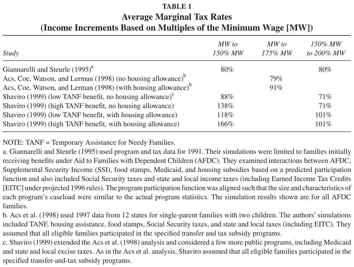
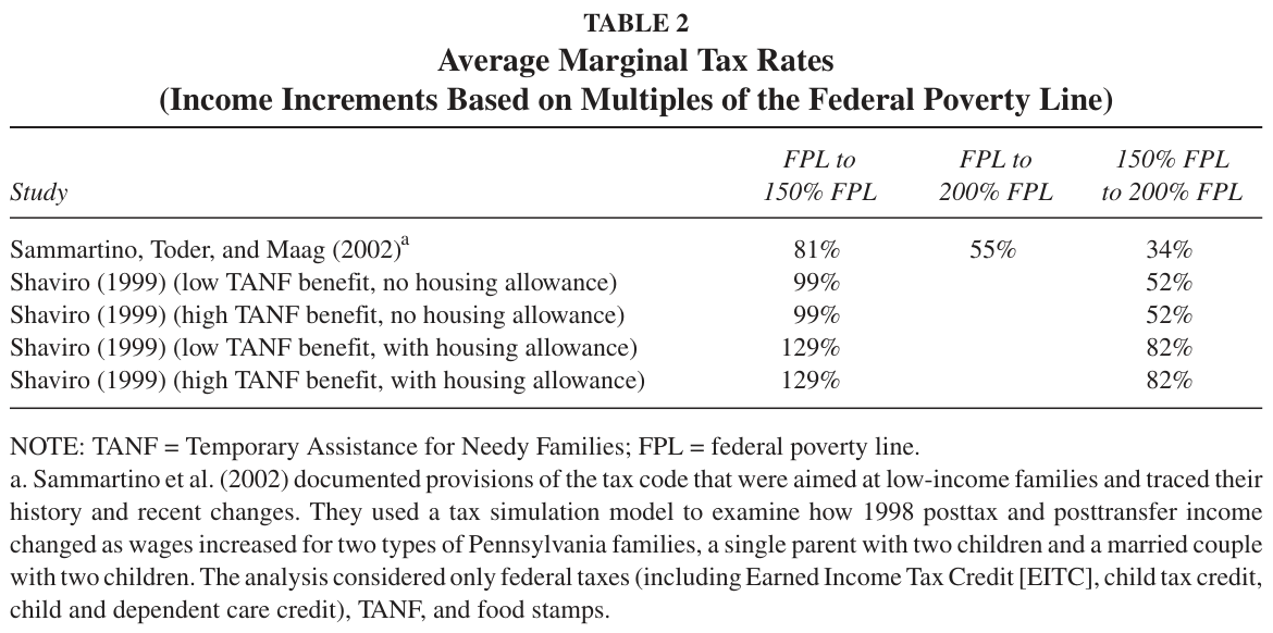
We know of no empirical estimates of the effect of high marginal tax rates on the ability of living wage laws to move working poor families out of poverty. The literature has focused primarily on the welfare population rather than the working poor and, as indicated above, has mostly ignored the implications of high marginal tax rates for wage mandates. However, the literature can provide us with a rough idea of how high marginal tax rates may be for families experiencing the types of wage increases mandated by living wage laws. In Tables 1 and 2, we summarize the marginal tax rates found in prior research averaged for an income range between the minimum wage and multiples of the minimum wage and between the federal poverty line and multiples of the federal poverty line, respectively. We adjusted the reported figures in Giannarelli and Steurle (1995), Sammartino et al. (2002), and Shaviro (1999) to be consistent with an assumption that the employer’s share of Social Security taxes was not part of the earnings base.1
### Table 1. Average Marginal Tax Rates (Income Increments Based on Multiples of the Minimum Wage [MW])
Table 1. Average Marginal Tax Rates (Income Increments Based on Multiples of the Minimum Wage [MW]) — source page 4. Open full-resolution image · Read source PDF page
**Notes:** NOTE: TANF = Temporary Assistance for Needy Families.
a. Giannarelli and Steurle (1995) used program and tax data for 1991. Their simulations were limited to families initially receiving benefits under Aid to Families with Dependent Children (AFDC). They examined interactions between AFDC, Supplemental Security Income (SSI), food stamps, Medicaid, and housing subsidies based on a predicted participation function and also included Social Security taxes and state and local income taxes (including Earned Income Tax Credits [EITC] under projected 1996 rules). The program participation function was aligned such that the size and characteristics of each program’s caseload were similar to the actual program statistics. The simulation results shown are for all AFDC families.
b. Acs et al. (1998) used 1997 data from 12 states for single-parent families with two children. The authors’ simulations included TANF, housing assistance, food stamps, Social Security taxes, and state and local taxes (including EITC). They assumed that all eligible families participated in the specified transfer and tax subsidy programs.
c. Shaviro (1999) extended the Acs et al. (1998) analysis and considered a few more public programs, including Medicaid and state and local excise taxes. As in the Acs et al. analysis, Shaviro assumed that all eligible families participated in the specified transfer-and-tax subsidy programs.
### Table 2. Average Marginal Tax Rates (Income Increments Based on Multiples of the Federal Poverty Line)
Table 2. Average Marginal Tax Rates (Income Increments Based on Multiples of the Federal Poverty Line) — source page 4. Open full-resolution image · Read source PDF page
**Notes:** NOTE: TANF = Temporary Assistance for Needy Families; FPL = federal poverty line.
a. Sammartino et al. (2002) documented provisions of the tax code that were aimed at low-income families and traced their history and recent changes. They used a tax simulation model to examine how 1998 posttax and posttransfer income changed as wages increased for two types of Pennsylvania families, a single parent with two children and a married couple with two children. The analysis considered only federal taxes (including Earned Income Tax Credit [EITC], child tax credit, child and dependent care credit), TANF, and food stamps.
. . . . the literature suggests that . . . high marginal tax rates can . . . impair the effectiveness of living wage mandates to improve family economic well-being.
The results displayed in the tables indicate that the marginal tax rates facing low-income families are quite high, particularly in an income range of up to 1.5 times the minimum wage or to 1.5 times the poverty line (in some instances greater than 100%). The rates are particularly high when families participate in multiple transfer or tax subsidy programs. Thus, the literature suggests that such high marginal tax rates can certainly impair the effectiveness of living wage mandates to improve family economic well-being. This is so even under the most favorable assumption that there is no employment displacement or reductions in hours as a consequence of the living wage law. Our analysis builds on this literature to examine more specifically the consequences of high marginal tax rates for the effectiveness of living wage laws in view of the mix of families likely to be affected and their participation in public transfer and tax subsidy programs.
### OBJECTIVES AND APPROACH
We investigated the significance of marginal tax rates on the economic well-being of households affected by living wage laws. First, we estimated schedules showing the relationship between household earnings and comprehensive disposable income (i.e., income after accounting for taxes and transfers, including welfare benefits, EITCs, and child tax credits) for various types of households in seven U.S. cities: Baltimore, Boston, Chicago, Detroit, Los Angeles, New York, and San Francisco. These cities were selected because they either have living wage laws or, in the case of New York City, have been targets of minimum wage campaigns. The income schedules for households differed by whether the household participated in public transfer and tax subsidy programs because such programs typically alter the relationship between gross before-tax earnings and net disposable income for the household. In computing the schedules, we considered the following transfer, tax, and tax subsidy programs for the selected cities: federal, state, and local income taxes; FICA taxes; tax credit programs (federal and state EITCs and the federal child tax credit;2 TANF; food stamps; and Section 8 housing assistance.3
For our living wage impact analysis, we drew a sample of individuals for 1999 using the 1996 panel of the Survey of Income and Program Participation (SIPP; U.S. Census Bureau, 1998a, 1998b). The appendix provides a description of the SIPP, including sample size information. In that sample, we identified a number of households in the seven cities that might be affected4 by universal coverage laws mandating a wage rate of at least $8.83.5
We assigned each of the “affected” households in the sample to particular schedules associating comprehensive disposable income (CDI) with gross earnings (GE).6 We then computed the change in GE and CDI associated with the increased wage income from the living wage mandate. Household GE without the wage mandate was computed as the reported household earnings. Household GE with the wage mandate was computed as the sum of the earnings for affected workers7 in the household (i.e., the reported hours of work times $8.83) plus the reported earnings for the unaffected workers. CDI (both with and without the wage mandate) was computed using household earnings, state and federal tax liability rules8 , and transfer program benefit determination rules.
We computed an average marginal tax rate (MTR) in 1999 for each sample household by the formula:
where the changes are measured between the household’s observed baseline GE and CDI and the GE and CDI associated with the living wage intervention. The MTR measures the fraction of the living wage–induced change in earnings that is kept by the household after taxes and loss of benefits are considered. The next section reports the computed MTRs for different groups of households for each of the seven cities examined.
We also conducted an analysis of the effect of the MTRs on the effectiveness of living wage laws in reducing the amount and degree of poverty in the seven cities. We did this by using two different measures of poverty, one based only on GE and the other based on CDI. We computed poverty for both income concepts using the federal poverty line (FPL) and 200% of the FPL. Poverty rates for our sample (with and without the living wage intervention) were computed by using the ratio of the number of households with income (GE or CDI) falling below the household’s own applicable poverty standard (FPL or 200% FPL). We also examined the rate at which poor households left poverty with and without the living wage intervention. We measured the extent of poverty (or the “poverty gap”) by examining the distance (in amount and percentage) between household income and the applicable poverty line, with and without the living wage intervention. The analysis based on GE essentially ignored the MTRs, whereas the analysis based on CDI showed the effect of the MTRs in limiting the antipoverty effectiveness of living wage laws.
### ANALYSIS OF THE LIVING WAGE USING THE SIPP
### Characteristics of Families With Low Wages From the SIPP
To assess the importance of high cumulative marginal tax rates resulting from multiple program participation, we examined microdata from the SIPP. As discussed in the appendix, we constructed a sample of nonelderly households that were followed for the calendar years 1996 to 1999. Overall, we followed 2,711 households, of which 44.7% were married with children, 16.3% were single-parent families, and 39% were childless. To maintain consistency with the analysis in the other sections, we took households that were initially in Baltimore, Boston, Chicago, Detroit, Los Angeles, New York, and San Francisco.
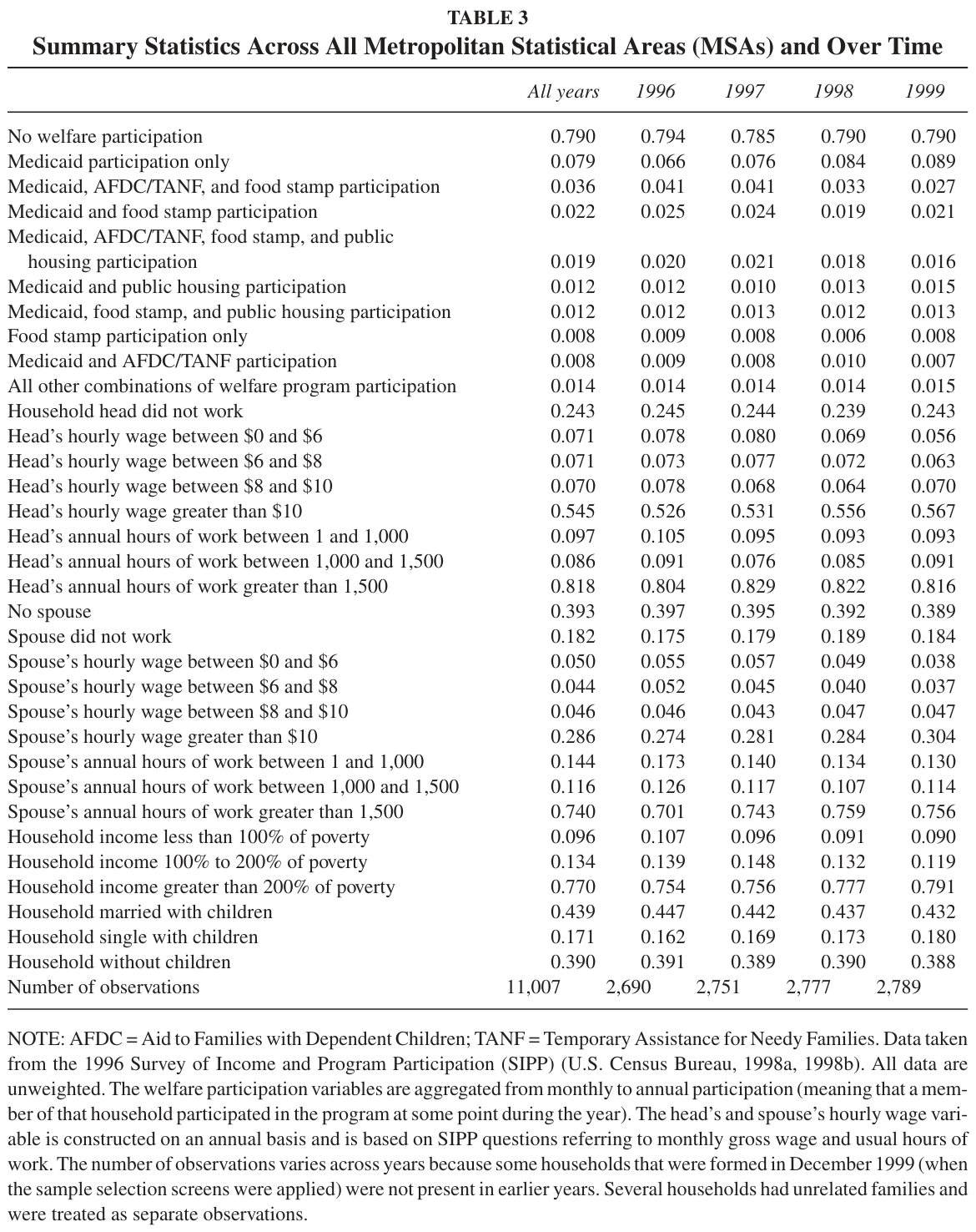
We examined overall program participation in Table 3 for all households, including nonearners. We present the tabulations for the 1996–1999 period as a whole and for each year separately to highlight major downward trends in program participation because of implementation of the Personal Responsibility and Work Opportunity Reauthorization Act (PRWORA) of 1996 and the improving economy. We defined welfare participation on an annual basis in these tables and found that across the entire sample, about 79% of households did not participate in Medicaid, Aid to Families with Dependent Children (AFDC)/TANF, public housing, or food stamps. The entire sample did not condition on low income or low wages, so participation was fairly low. Interesting, even with the improving economy and welfare reform, participation in no welfare programs remained fairly stable from 1996 to 1999, as seen in Table 4. The next nine rows of Table 4 break out participation in different kinds of welfare programs. The single largest category for welfare participation is Medicaid. Unlike other welfare programs, such as AFDC/TANF or food stamps, which were being scaled back during this period, Medicaid was expanding because of the phasing in of Medicaid changes from the late 1980s and early 1990s and because of the implementation of the State Children’s Health Insurance Program (SCHIP) in the late 1990s. Overall, 18.8% of households participated in Medicaid, either alone or in conjunction with another program. The percentage of families in these metropolitan statistical areas (MSAs) that participated in Medicaid alone increased from 6.6% to 8.9%. However, for the sample as a whole, multiple program participation was quite common. With the exception of Medicaid (which currently has very generous income limits), less than 1% of households participated only in AFDC/TANF, food stamps, or public housing.
The remaining rows show breakdowns by the household head’s and spouse’s hourly wage rate, by poverty status, and by the distribution of family structures. Wage rates were computed by dividing annual earnings by annual hours of work. In about 25% of the households, the head had no reported earnings or hours in a given year, so it was not possible to compute his or her hourly wage rate. About 21% of household heads had an imputed hourly wage rate less than $10 per hour, and 54% had wage rates greater than $10 per hour. Almost 40% of the sample was unmarried, and nearly 20% had a nonworking spouse. Working spouses who earned less than $10 per hour constituted 14% of the sample, whereas working spouses who earned more than $10
per hour made up 29% of the sample. In our sample, about 9% lived in poverty in a given year (based on gross income), and another 14% had family income under 200% of the poverty line.
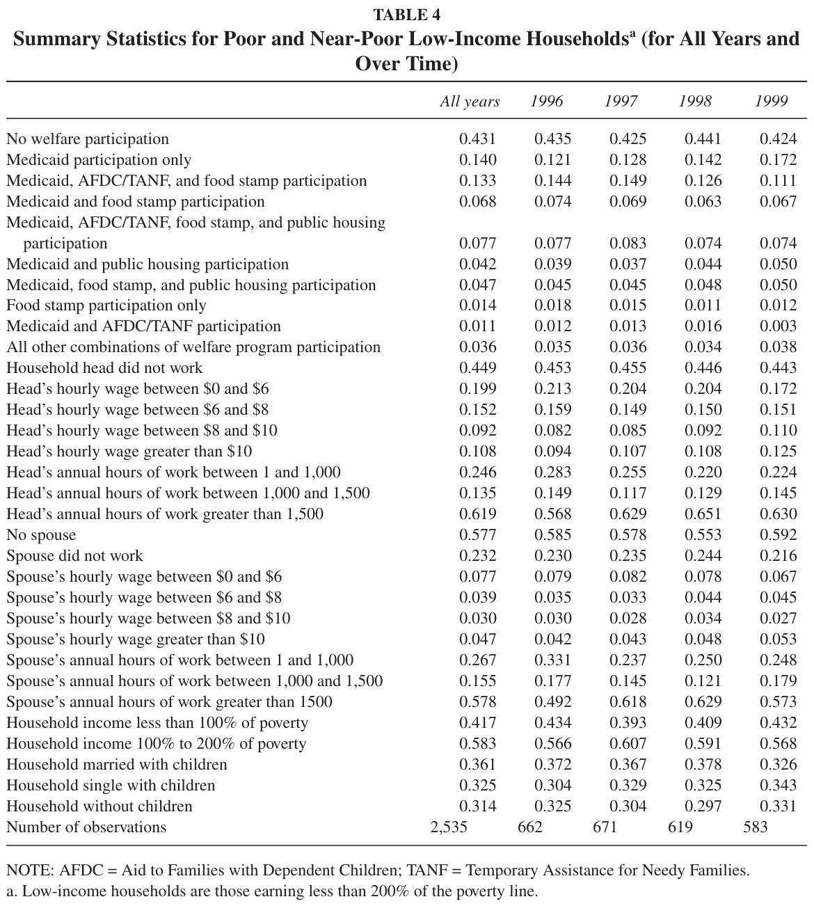
Table 4 breaks out welfare participation by family income by showing participation rates for the “near poor” with incomes less than 200% of poverty. Clearly, the patterns of program participation were much more dramatic. More than half of poor and near-poor families participated in welfare. Of those who participated, about one third participated only in Medicaid, and most of those remaining participated in multiple programs. More than 13% of poor and near-poor households participated in Medicaid, AFDC/TANF, and food stamps, and more than 7% participated in Medicaid, AFDC/TANF, food stamps, and public housing. It is important to note that there are often long waits to enter public housing, so presumably, some households that were not participating would participate if they could get in. Again, with the exception of Medicaid, participation in only one welfare program was not very common. Briefly examining the other rows shows, as one would suspect, that the labor force participation rate was much lower for poor households, and conditional on work, the wage distribution was much lower. About 45% of poor households had a head with no earnings, and about 45% had a head who earned less than $10 per hour. Thus, this group was very likely to be affected by living wage laws and had high participation rates in multiple welfare programs.
Simulating the Effects of the Living Wage: Preliminaries This section reports on simulations of the effect of a living wage increase to $8.83 per hour, the median for living wage localities through 1999. A living wage of this level equates to annual earnings of $17,660 for a full-time, full-year worker. For each city where the SIPP data were examined, we included observations that met the following criteria: (a) the data were from 1999 only, (b) either the head or spouse initially had a wage rate between the minimum wage and the new living wage, and (c) families who reported receipt of a welfare program but were deemed statutorily ineligible by our imputation were excluded. The second and third screens reduced the sample from 2,711 households to 420 households. Our simulation, therefore, included families who may not have been in poverty (because only one of the two earners needed to be affected). If both the head and spouse were affected, both wage rates were increased to $8.83 per hour.
### Table 3. Summary Statistics Across All Metropolitan Statistical Areas (MSAs) and Over Time
Table 3. Summary Statistics Across All Metropolitan Statistical Areas (MSAs) and Over Time — source page 7. Open full-resolution image · Read source PDF page
**Notes:** NOTE: AFDC = Aid to Families with Dependent Children; TANF = Temporary Assistance for Needy Families. Data taken from the 1996 Survey of Income and Program Participation (SIPP) (U.S. Census Bureau, 1998a, 1998b). All data are unweighted. The welfare participation variables are aggregated from monthly to annual participation (meaning that a member of that household participated in the program at some point during the year). The head’s and spouse’s hourly wage variable is constructed on an annual basis and is based on SIPP questions referring to monthly gross wage and usual hours of work. The number of observations varies across years because some households that were formed in December 1999 (when the sample selection screens were applied) were not present in earlier years. Several households had unrelated families and were treated as separate observations.
The analysis focused on each earner’s total annual wages and the family’s tax status (head of household, single, or married).9 Program benefits for food stamps, TANF, and Section 8 were calculated, as well as federal, state, and local taxes, and employment taxes (such as Social Security and Medicare). All families’ earnings, income, and marginal tax rates were modeled on the basis of their reported program participation and estimated welfare benefits. We assumed that all households filed a tax return and claimed the standard deduction.
Although few families received all their income from welfare benefits, as we noted earlier, many participated in one program or another during a given year. The cumulative marginal tax rate for each household was determined by adding the marginal tax rates for the programs in which the household participated. In all of the following analyses, we assumed no behavioral responses to the living wage. In particular, we assumed that hours worked and labor force participation were unaffected by the change in the wage rate. If the living wage had disemployment effects, the following analysis would overestimate the effect on moving out of poverty.
### Table 4. Summary Statistics for Poor and Near-Poor Low-Income Households (for All Years and Over Time)
Table 4. Summary Statistics for Poor and Near-Poor Low-Income Households (for All Years and Over Time) — source page 8. Open full-resolution image · Read source PDF page
**Notes:** NOTE: AFDC = Aid to Families with Dependent Children; TANF = Temporary Assistance for Needy Families.
a. Low-income households are those earning less than 200% of the poverty line.
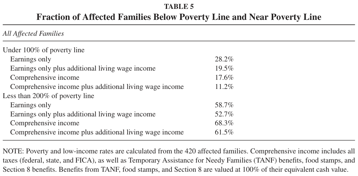
### Table 5. Fraction of Affected Families Below Poverty Line and Near Poverty Line
Table 5. Fraction of Affected Families Below Poverty Line and Near Poverty Line — source page 9. Open full-resolution image · Read source PDF page
**Notes:** NOTE: Poverty and low-income rates are calculated from the 420 affected families. Comprehensive income includes all taxes (federal, state, and FICA), as well as Temporary Assistance for Needy Families (TANF) benefits, food stamps, and Section 8 benefits. Benefits from TANF, food stamps, and Section 8 are valued at 100% of their equivalent cash value.
. . . it is clear that the living wage was not well targeted on the poor.
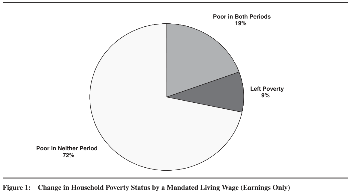
### Figure 1. Change in Household Poverty Status by a Mandated Living Wage (Earnings Only)
Figure 1. Change in Household Poverty Status by a Mandated Living Wage (Earnings Only) — source page 9. Open full-resolution image · Read source PDF page
**Caption:** Change in Household Poverty Status by a Mandated Living Wage (Earnings Only).
### The Effect of the Living Wage on Poverty Rates
The first general question is, Does the living wage reduce poverty? In general, we used two different income bases for determining poverty rates: One base relied solely on the household head’s and spouse’s earnings, and the second relied on CDI. CDI adds earnings, the EITC, and welfare benefits and subtracts taxes. In-kind benefits are assumed to be worth the same as cash. An analysis that focuses only on earnings and ignores the tax rates from the tax and transfer system is akin to an analysis that assumes a 0% tax rate.
Figures 1 and 2 and Table 5 examine the effects of the living wage on poverty rates using the SIPP (in the remaining sections, household weights are used). When one focuses on the figures, it is clear that the living wage was not well targeted on the poor: The overwhelming majority (72%) who benefited were not poor before the simulation. Of the 28% of households that were initially poor before the simulation, about one third left poverty.
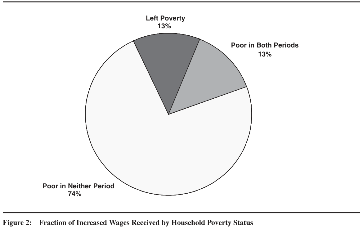
It could be conjectured that even though most who were affected by the living wage were not poor, the total expenditure disproportionately benefited those below the poverty line. For example, if most of the nonpoor in Figure 1 had earners concentrated just below the $8.83 living wage and if most of the poor had earners concentrated near the minimum wage, then the bulk of the expenditure would be, in fact, well targeted. However, Figure 2 shows that this is not the case: The nonpoor received a nearly identical amount (74%) of the expenditure. Although those who were not poor initially had higher wage rates (which would reduce the effect of the living wage), they also had higher annual hours of work (which would increase the effect). Overall, the only striking difference between Figures 1 and 2 is that those who left poverty received a slightly higher proportion of the total expenditure, which suggests they worked more hours than those who remained poor.
### Figure 2. Fraction of Increased Wages Received by Household Poverty Status
Figure 2. Fraction of Increased Wages Received by Household Poverty Status — source page 10. Open full-resolution image · Read source PDF page
**Caption:** Fraction of Increased Wages Received by Household Poverty Status.
Table 5 shows several additional calculations. The reduction in poverty rates was 8.7 percentage points when tax rates from the tax-and-transfer system were ignored. As the third and fourth rows show, both the initial level and the reduction were smaller after these taxes were accounted for. The initial poverty rate, 17.6%, was almost 40% lower using CDI, and the reduction in poverty was 6.4 percentage points, only about three fourths of the effect that ignored tax rates.
The second set of rows examines an alternative measure—whether the family was “poor” or “near-poor” (i.e., having income under 200% of the poverty line). Strikingly, 41% of the sample was neither poor nor near-poor before the living wage increase, and our tabulations show that this group received 39% of the total expenditure from the living wage increase. When we used CDI, a smaller proportion was above 200% of the poverty line because most households were ineligible for welfare benefits around that level and the taxes reduced a family’s gross income to under this threshold. In both cases—using earnings alone (and assuming a 0% tax rate) or CDI (and assuming a realistic tax rate)—the reduction in the number of households with income below 200% of the poverty line was approximately 6 to 7 percentage points. This suggests that the focus on marginal tax rates is less relevant for higher income thresholds, although important differences emerge around the poverty line.
### The Effect of the Living Wage on Income
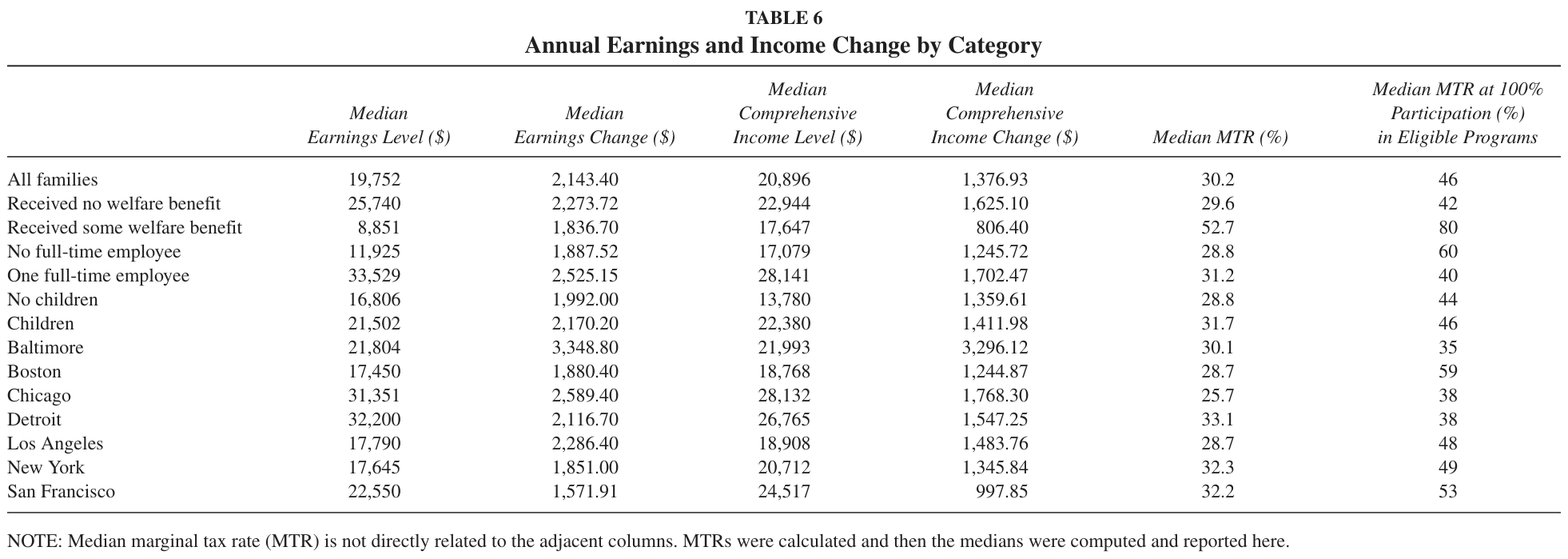
Table 6 breaks out the analysis by region and demographics and illustrates the differences in income changes and tax rates for these groups. Overall, the median earnings for the 420 households affected by the living wage were $19,752, whereas median comprehensive income was about $1,000 higher. Moving down the table, one sees, as expected, enormous differences in median earnings for welfare and nonwelfare recipients (about $17,000). The difference in comprehensive income is much smaller (about $5,000), showing the importance of accounting for the tax-and-transfer system. Large income differences emerge based on full-time work status, although the gap is again closed when examining comprehensive income levels. The table also shows that families with children have higher earnings (reflecting, in part, higher marriage rates and higher ages of the household head). These differences do not narrow with comprehensive income, reflecting the fact that many subsidies (welfare and EITC) are largely targeted toward families with children.
### Table 6. Annual Earnings and Income Change by Category
Table 6. Annual Earnings and Income Change by Category — source page 11. Open full-resolution image · Read source PDF page
**Notes:** NOTE: Median marginal tax rate (MTR) is not directly related to the adjacent columns. MTRs were calculated and then the medians were computed and reported here.
Finally, there are large differences in earnings across metropolitan areas (although the sample sizes for some regions are relatively small, so the medians may be imprecisely estimated). Interesting, the interregion differences shrink considerably when CDI is examined.
Overall, the MTR [marginal tax rate] for those affected by the living wage is 30.2%. Table 6 also shows changes in median earnings and median CDI, as well as median (average) MTRs. Note that the median MTRs do not exactly correspond to 1 minus the ratio of change in median CDI to change in median earnings, because MTRs are calculated for each individual and then the median MTR is taken. In general, there is more variability in the comprehensive income change than in the earnings change. The earnings change ranges from $1,572 to $3,349 (with most changes around $2,000), whereas the income change ranges from $806 to $3,296. There are several noteworthy differences in MTRs. Overall, the MTR for those affected by the living wage is 30.2%. Those on welfare face substantially higher MTRs (53% vs. 30%). This finding itself is unsurprising because food stamps and housing each have MTRs of 30%, and TANF can potentially have an MTR of 100%. Low take-up rates of some of the program combinations by the median household keeps the MTR as low as it actually is (as well as subsidies from the EITC). This is reinforced by examining the last column, which assumes 100% program participation among eligible households. In this case, the MTR is 80%, but our analysis shows that such a 100% take-up assumption is far from the truth.
MTRs vary little by full-time work status or by the presence of children. This can be explained for full-time work by the fact that many full-time workers are in the EITC phase-out range (with a tax rate of 21%), while part-time workers are often in the subsidy range (with a 40% subsidy), which offsets the high MTRs of welfare programs. Similarly, although families with children have higher participation in welfare programs (which adds to the cumulative MTR), they often get the EITC, which may reduce the MTR. Finally, the analysis shows that median MTRs do not vary much by metropolitan area, but if 100% program take-up is assumed, there is considerably more variation.
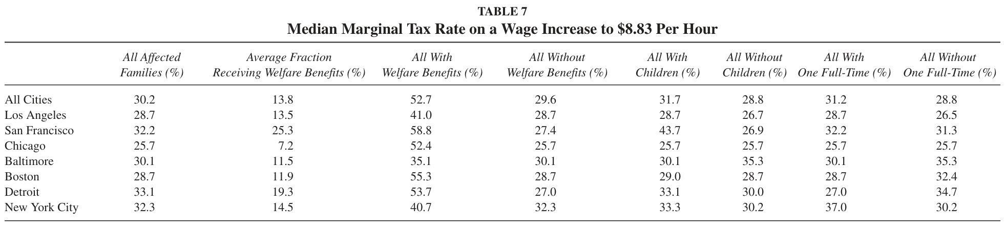
The lack of regional variation is perhaps surprising, given the diversity of metropolitan areas in terms of their social safety nets and state and local tax systems. Table 7 explores these differences further, with the first column replicating the MTRs from Table 6. The second column shows participation rates in any welfare program (TANF, food stamps, or public housing). It is apparent that the lack of variation in the overall sample hides the fact that there is large variation in both take-up rates and MTRs conditional on take-up. The participation rate is as low as 7% in Chicago and as high as 25% in San Francisco. When MTRs are examined by take-up in any program versus no take-up, MTRs vary by as many as 18 percentage points for welfare participants but fewer than 7 percentage points for nonparticipants. Similar tabulations were done by metropolitan area for families with and without children and by full-time work status. The variation in MTRs by children is, again, largely driven by differences in take-up of welfare benefits, whereas there is not much variation in MTRs by full-time work status.
### The Effect of the Living Wage on the Poverty Gap
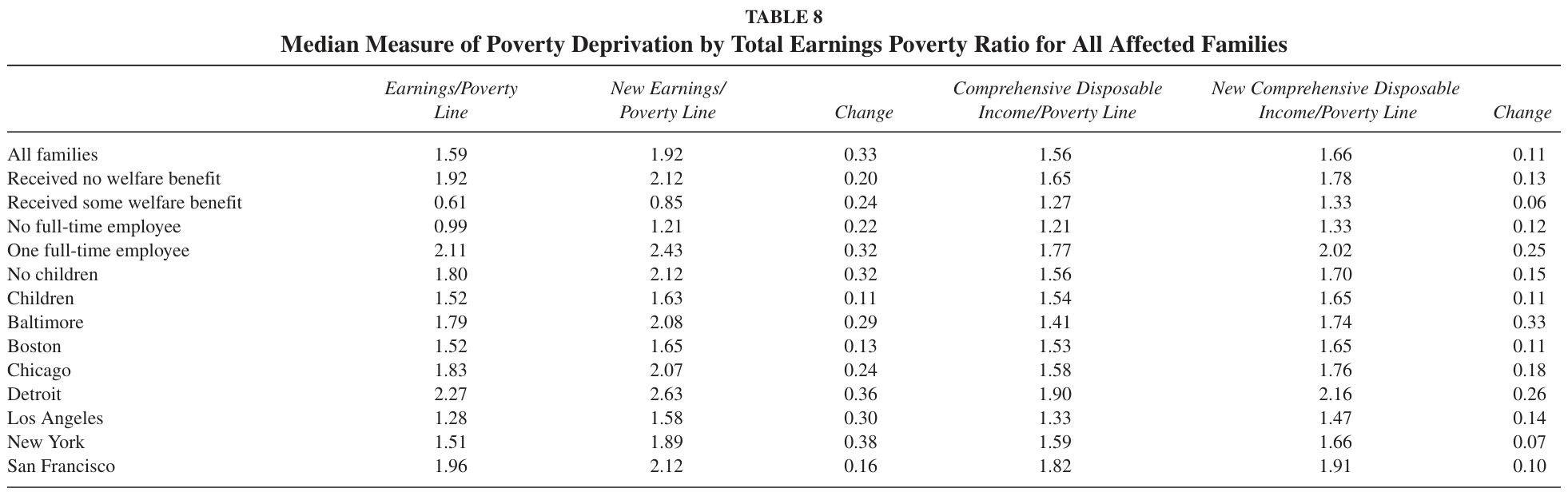
The final three tables (Tables 8, 9, and 10) consider effects of living wage ordinances on income in relation to poverty on low-income thresholds. The poverty ratio, defined in Table 8 as the ratio of earnings and CDI to the family’s poverty line, was about 1.6 before simulating the effects of the living wage. This means that a typical family in our sample had earnings nearly 60% higher than the poverty line before a wage increase. A number below 1.00 indicates that the median family in the sample was in poverty, such as those who received some welfare benefit.
It is expected that giving all families a substantial wage increase (and ignoring disemployment effects) will yield substantial changes in earnings and CDI. Comparing the third and sixth columns of Table 8 shows there is a substantial difference in how typical families fare when considering the “total earnings poverty ratio” to the “total income poverty ratio.” Although the initial levels are very similar for all families, the change is three times larger for earnings than for CDI. This again emphasizes the importance of the MTRs from the tax and transfer system. Moving down the columns, one can observe that in almost all scenarios, the “true” change in well-being is overstated by ignoring MTRs. One might expect those on welfare (the third row) to have essentially zero change in their well-being for CDI but a large change for earnings. As it turns out, the change for earnings is about the same as for nonwelfare recipients, whereas the change in comprehensive income is indeed very small. The reason that earnings do not change very much in column 3 is the small number of hours worked.
### Table 7. Median Marginal Tax Rate on a Wage Increase to $8.83 Per Hour
Table 7. Median Marginal Tax Rate on a Wage Increase to $8.83 Per Hour — source page 13. Open full-resolution image · Read source PDF page
### Table 8. Median Measure of Poverty Deprivation by Total Earnings Poverty Ratio for All Affected Families
Table 8. Median Measure of Poverty Deprivation by Total Earnings Poverty Ratio for All Affected Families — source page 13. Open full-resolution image · Read source PDF page
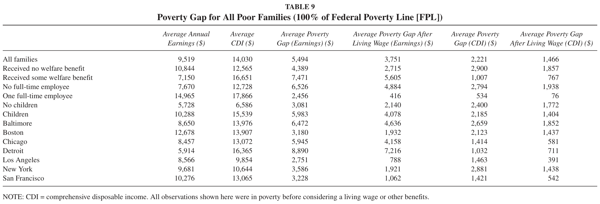
### Table 9. Poverty Gap for All Poor Families (100% of Federal Poverty Line)
Table 9. Poverty Gap for All Poor Families (100% of Federal Poverty Line) — source page 14. Open full-resolution image · Read source PDF page
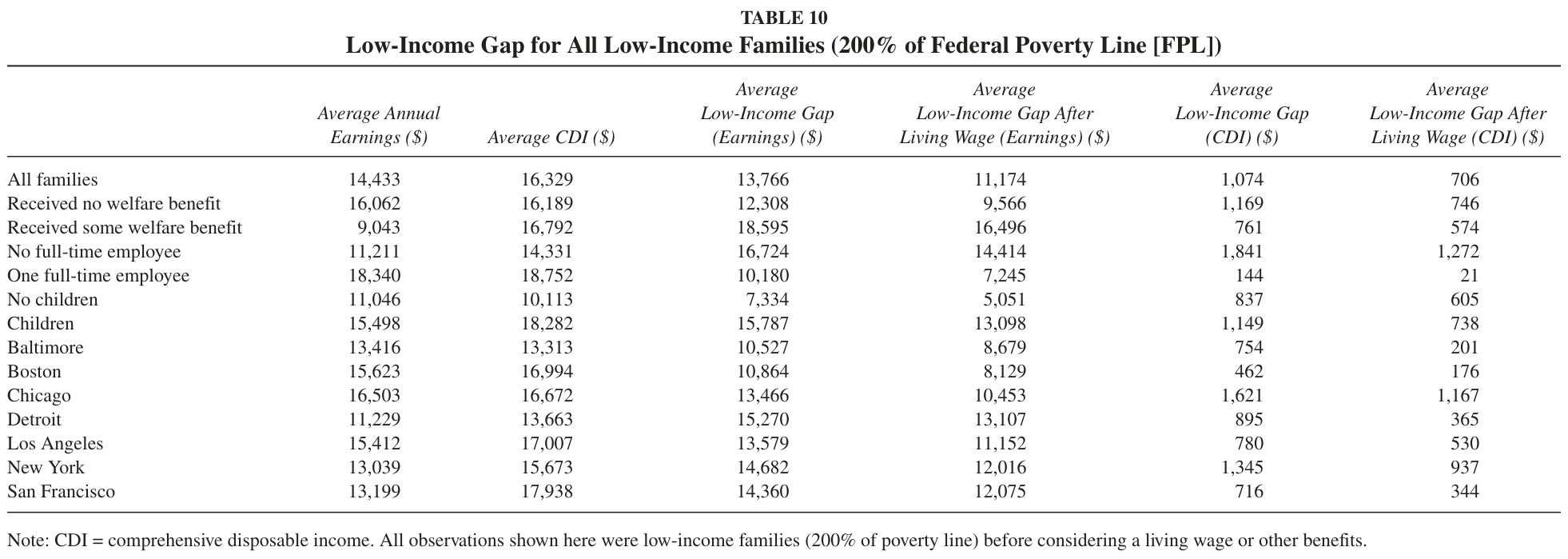
As illustrated in Figure 1 and Table 5, the living wage largely benefits those who are not initially poor. It is still useful, perhaps, to see whether conditional on being in poverty (or near poverty), the living wage has much effect. The analyses in Tables 9 and 10 examine the “poverty gap” and the “near poverty gap.” The poverty gap is defined for families as the difference between the poverty line and their actual earnings or income (and would be zero for families above the poverty line). The sample in Table 9 consists of those who were in poverty (based on earnings or CDI) before the living wage increase, whereas Table 10 expands the sample to those with incomes less than 200% of the poverty level. For poor families in Table 9, annual household earnings were $9,519, or $5,494 below the poverty line, on average. CDI was substantially higher ($14,030) with a much smaller poverty gap of $2,221. Note that the composition of families is different across the columns (based on the definition of poverty), so the actual poverty line varies by column.
As the fourth and sixth columns show, the general conclusions about the effectiveness of the living wage depend critically on accounting for the consequences of the tax-and-transfer system. The change in the poverty gap based on earnings is fairly substantial ($1,700) but is much smaller based on CDI ($750). These differences emerge by work status, family structure, and region. The robust finding from Table 9 is that the effect of the living wage on economic well-being is quite small for those in poverty. Finally, Table 10 recalculates these numbers for the “near-poverty” gap. The same kinds of conclusions emerge here. The near-poverty gap falls by $2,600 for all families based on earnings but only by $300 based on CDI. Again, the effect of the living wage on well-being appears to be quite modest for those who are the worst off.
## CONCLUSION
This article has explored the consequences of implementing a living wage law on the economic status of affected households. Absent from the usual discussion about the effect of such living wage laws are the high cumulative marginal tax rates present in means-tested programs, such as AFDC/TANF, food stamps, and public housing, and in the phase-out range of the EITC. These welfare programs disproportionately affect single-parent households, but some programs are also available for married households with children and households without children.
The cumulative MTR, after these programs are included, is very high and may exceed 100% for some income ranges, which implies that the implementation of living wage laws may not improve the well-being of the affected households. The analysis here focuses on several large metropolitan areas, most of which could be considered as having high costs of living. The results of living wage laws that apply to these MSAs are likely to apply to areas with lower costs of living, too. AFDC/ TANF is a state-level program, food stamps is national, and the income limits for public housing are almost always in the relevant range for the currently proposed living wage laws. We show that for many families, especially those who have low annual incomes or low hourly wage rates, welfare participation is quite common and multiple program participation is the rule, not the exception.
Although beyond the scope of the current study, there are several other relevant transfers that could be considered. We did not include Supplemental Security Income, which offers assistance to poor households with disabled adults or children. We excluded energy assistance, which is means-tested and tends to vary at the local level. We also ignored child-care subsidies, school breakfast and lunch programs, and Head Start. All of these are means-tested as well and, for at least some of the families in the sample, would increase the tax rates even more. Finally, it was beyond our scope to incorporate Medicaid (because it currently has income limits for many families that are well beyond those of proposed living wage laws). Over some income ranges, the loss of Medicaid would produce an exorbitant MTR because of the “notch” in the budget constraint (Yelowitz, 1995, 2000).
### Table 10. Low-Income Gap for All Low-Income Families (200% of Federal Poverty Line [FPL])
Table 10. Low-Income Gap for All Low-Income Families (200% of Federal Poverty Line [FPL]) — source page 16. Open full-resolution image · Read source PDF page
**Notes:** Note: CDI = comprehensive disposable income. All observations shown here were low-income families (200% of poverty line) before considering a living wage or other benefits.
Proponents of living wage laws seem to be aware that the high tax rates make it difficult for such wage mandates to significantly increase family income. However, they argue that having a higher paying job leads to improvements in workers’ self-esteem and even productivity. However, such psychological benefits would seem to be a kind of psychic illusion, with the worker assumed to be blind to the regulatory manipulation of market wages. However, this illusion, if it exists, is not innocuous, because workers may be led away from socially beneficial investments in education and training, and even geographic mobility, by their belief that their wages may remain high even without the additional human capital investment. Also, workers may learn, to their dismay, that they are trapped in living wage jobs that pay wages well above their next-best alternatives outside the jurisdiction of the living wage laws. If society wants to improve the economic status of low-income families, it seems to us that the best way to do this is through targeted tax credits that go to families most in need and do not trigger either additional taxes or losses in benefits from public programs.10
Our study suggests several directions for future research. First, our simulations suggest that the effect of living wage laws on family income should be very modest. Given the phase-in of living wage laws from 1994 onward, it should be possible to use panel data to assess the empirical effect of these laws on total income and welfare income. Second, eligibility, taxes, and benefits for welfare programs are most often determined monthly, whereas federal income taxes are determined annually. This opens up the possibility of “bunching” earnings into several months of the year and welfare benefits into other months of the year. By doing so, a household strategically could avoid some of the high MTRs because the earnings would be zero during the months the household was on welfare. Finally, our analysis suggests the incidence of the living wage should vary by family structure. Childless households tend to benefit the most from living wage laws because they are ineligible for most welfare benefits, whereas single-parent households tend to benefit the least. Using the actual implementation of the laws, one can explore whether these predictions hold up.
### APPENDIX Survey of Income and Program Participation (SIPP) Data Analysis
The SIPP analysis uses information from the 1996 panel, which consisted of 40,000 households who were interviewed 12 times between April 1996 and March 2000 (U.S. Census Bureau, 1998a, 1998b). The SIPP contains basic demographic and social characteristics data for each member of the household. These include age, sex, race, ethnic origin, marital status, household relationship, education, and veteran status. Core questions, which are repeated in each interview, cover labor force activity, types and amounts of income, and participation in various cash and noncash benefit programs for each month of the 4-month reference period. Data for employed people include number of hours and weeks worked, earned income, and weeks without a job. Core data also cover postsecondary school attendance, public or subsidized rental housing, low-income energy assistance, and school breakfast and lunch participation.
The sample in each wave consists of four rotation groups, each interviewed in a different month. For Wave 1, the interview months were from February 1996 to May 1996. For each group, the reference period for reporting labor force activity and income is the 4 calendar months preceding the interview month. Thus, the information for a household started anywhere between October 1995 and January 1996.
The SIPP is a longitudinal survey where each sampled household and each descendant household is reinterviewed at 4-month intervals for 12 interviews or “waves.” Unique codes were included on each record to allow linking together the same people from the preceding and subsequent waves.
The SIPP’s geographic coverage is the United States, and codes are included for 41 individual states and the District of Columbia, although the sample was not designed to produce state-representative estimates. Areas of the SIPP sample in nine other states were identified in groups for confidentiality reasons. The file identifies a subsample of metropolitan residents, along with codes for selected metropolitan statistical areas (MSAs) and consolidated metropolitan statistical areas (CMSAs). SIPP can shed light on living wage and MTR issues. The SIPP collected the source and amount of income, labor force information, program participation and eligibility data, and general demographic characteristics to measure the effectiveness of existing federal, state, and local programs. It sampled the U.S. civilian noninstitutionalized population. The SIPP content was built around a “core” of labor force, program participation, and income questions designed to measure the economic situation of people in the United States. It interviewed households every 4 months, asked retrospective questions on a monthly basis, and followed households for up to 48 months. A new cohort was introduced each year, forming a new “panel.” From the 1996 panel, all “person-months” were obtained from all 12 waves. We then applied a number of screens. First, we defined the household head’s age, MSA of residence, and family structure in the December 1999 interview month. This was done because our analysis examined living wage changes in 1999, and the federal tax code defines a family unit as of December 31 of each year. One quarter of the SIPP sample had their last interviews in November 1999, so the age, MSA, and family structure variables were taken from that month for them.
The sample initially consisted of 3,897,232 “person-months” on 44,047 households. We kept observations only from “living wage” MSAs (and our “control” MSA). We therefore selected household heads who were initially living in Baltimore, Boston, Chicago, Detroit, Los Angeles, New York, and San Francisco. We eliminated households that were not living in one of these MSAs as of December 1999, which reduced the sample to 3,851 households. Next, we kept households that had a head aged 15 to 64 (inclusive), which reduced the sample to 2,711 households and largely eliminated households with elderly heads. Next, we restricted the data to the calendar years 1996 to 1999 and kept observations on household heads. The final sample consists of 129,791 “person-months” on 2,711 households.
Some of our tables divide the 2,711 households by the head’s (and spouse’s) hourly wage rate or hours of work. In our data, we imputed an hourly wage rate for each person as follows: For each calendar year, we aggregated earnings and hours from the month to annual level and then divided annual earnings by annual hours.
## Printed notes
**1.** This adjustment was made by multiplying the average marginal tax rate (MTR) by 1.0765 (to change the earnings base) and subtracting 0.0765 (to remove the employer’s share of payroll taxes). It was not necessary to adjust the estimated MTRs in Acs, Coe, Watson, and Lerman (1998) because they did not consider the employer’s share of payroll taxes as part of the earnings base and did not count the employer tax in computing MTRs. Tax incidence theory suggests that employees pay the employer’s share of the tax, and therefore, it should be included in gross income. However, when an employee’s wage increases because of a wage mandate, it will generally not be possible for the employer to shift the employer’s share of Social Security taxes to the employee by lowering his wage. Although the employer may find other ways to adjust to the higher labor costs, such as cutting employment and reducing hours, we have not considered such adjustments in this article.
**2.** Federal and state taxation rates, schedules, deductions, and credits were obtained from individual state and federal tax forms and instructions for 1999. For all federal and state tax calculations, standard deductions were used and included child tax credits, Earned Income Tax Credits (EITC) (both federal and state, where applicable) and household credits (as in the case of New York State, where families can receive both credits from the state and New York City). Not included in calculations were deductions for Child and Dependent Care, which are separate from child tax credits and are linked to expenditures on child or dependent care.
**3.** The rules for Temporary Assistance for Needy Families (TANF) were obtained from state welfare offices and Web sites. The food stamp rules were taken chiefly from the United States Department of Agriculture Web site (http://www.fns.usda.gov/fsp/applicant_recipients/fs_Res_Ben_Elig.htm). The 1999 benefit schedules and eligibility were obtained from http://www.dss.cahwnet.gov/getinfo/acl99/99-71.PDF . We assumed that the shelter allowance was equal to Housing and Urban Development’s (HUD) fair-market rent for the applicable area for the minimum size suggested by HUD. By these standards, a single adult would not need any more than a single room, and families with children would live in homes with one bedroom for every two children and one bedroom for parents (U.S. Housing and Urban Development, 2001). The fair-market rents for Section 8 were obtained from HUD at http://www.huduser.org/datasets/fmr99/incfy1999.xls.
**4.** We limited the sample to individuals who in 1999 earned between the maximum of the federal or state minimum wage and the living wage standard of $8.83 per hour, and we excluded people who reported public benefits (TANF, food stamps or Section 8 housing assistance) but who appeared to be statutorily ineligible. These screens reduced the Survey of Income and Program Participation (SIPP) sample to 420 households.
**5.** The hourly wage of $8.83 is the median living wage standard from about 40 local jurisdictions that had passed such laws by the end of 1999. Data on living wage laws were drawn from Employment Policies Institute (2002). Our analysis simulated the effect of a universal law covering all workers within a particular metropolitan statistical area (MSA). This is a fair test of whether a living wage ordinance can affect poverty in a local area. The actual laws are generally thought to have too narrow coverage to have any significant effect on poverty. Moreover, examining a law based on universal coverage allows us to analyze effects for the cities in our sample that already had living wage laws in effect in 1999 (all but New York City) because our simulations greatly expand the coverage of such actual laws.
**6.** As household gross earnings increase, comprehensive disposable income (CDI) changes by the amount of the earnings increase less the amount of additional taxes and less the amount of transfers lost. The slope of the schedule is the MTR, and the average slope during a particular range of earnings is the average MTR.
**7.** An affected worker was one whose reported hourly wage was between the applicable state minimum wage and $8.83. An unaffected worker was one whose reported wage fell outside this range or who reported no earnings.
**8.** We used federal and state tax schedules for 1999, assuming that all filers took the standard deduction. Married couples were assumed to file jointly. Unmarried household heads with children under 18 were assumed to file as heads of households. All others were assumed to file as singles.
**9.** Same as Number 8.
**10.** Two of us have argued elsewhere that a locally administered EITC is a more efficient way to raise the incomes of the working poor than is a wage mandate (Toikka & Neveu, 2002).
## References
Acs, G., Coe, N., Watson, K., & Lerman, R. (1998, July). _Does work pay? An analysis of the work incentives under TANF_ . Washington, DC: Urban Institute.
Employment Policies Institute. (2002). _Living wage proposals_ . Retrieved November 1, 2002, from www.livingwage.org
Giannarelli, L., & Steuerle, E. (1995). _The twice-poverty trap: Tax rates faced by AFDC recipients_ . Washington, DC: Urban Institute.
Pollin, R., & Luce, S. (1998). _The living wage: Building a fair economy_ . New York: New Press.
Sammartino, F., Toder, E., & Maag, E. (2002). _Providing federal assistance for low-income families through the tax system: A primer_ . Washington, DC: Urban Institute.
Shaviro, D. (1999). _Effective marginal tax rates on low-income households_ . Washington, DC: Employment Policies Institute.
Toikka, R., & Neveu, A. (2002). A local Earned Income Tax Credit: A better anti-poverty policy than wage mandates. _The Georgetown Public Policy Review_ , _8_ (1), 29-49.
U.S. Census Bureau. (1998a). _Survey of Income and Program Participation (SIPP) 1996 panel computer file: ICPSR version_ . Washington, DC: Author.
U.S. Census Bureau. (1998b). _Survey of Income and Program Participation (SIPP) 1996 panel Wave 1 core microdata files technical documentation_ . Washington, DC: Author.
U.S. Department of Housing and Urban Development. (2001). _Housing choice voucher program guidebook_ . Retrieved August 11, 2003, from http://www.hud.gov/offices/pih/programs/hcv/forms/guidebook.cfm.
Yelowitz, A. (1995). The Medicaid notch, labor supply, and welfare participation: Evidence from eligibility expansions. _Quarterly Journal of Economics_ , _110_ (4), 909-939.
- Yelowitz, A. (2000). _Evaluating the effects of Medicaid on welfare and work: Evidence from the past decade_ . Washington, DC: Employment Policies Institute.