# Racial climate and homeownership

**Authors:** Timothy F. Harris and Aaron Yelowitz<sup><a href="#source-note-1" aria-label="Source note 1">1</a></sup>  
**Affiliations:** Timothy F. Harris — Department of Economics, Illinois State University, College of Arts and Sciences, Stevenson Hall 425, Normal, IL 61790, United States; Aaron Yelowitz — Department of Economics, University of Kentucky, Gatton College of Business and Economics, 550 South Limestone Street, Lexington, KY 40506, United States.  
**Corresponding author:** Aaron Yelowitz (aaron@uky.edu). Timothy F. Harris: tfharr1@ilstu.edu.  
**Citation:** Timothy F. Harris and Aaron Yelowitz (2018). Racial climate and homeownership. Journal of Housing Economics 40: 41–72. DOI: 10.1016/j.jhe.2017.12.003.

Received 31 May 2017; received in revised form 12 December 2017; accepted 13 December 2017; available online 22 December 2017.

© 2017 Elsevier Inc. All rights reserved.  

## Abstract

An important question aside from outright discrimination is whether poor underlying race relations in an area might create a chilling effect on homeownership for minorities. From 2012 onward, there were a series of high-profile events in the U.S. related to police brutality which highlighted racial tension. Using Google Trends, we characterize a locality’s underlying racial climate based on search interest in these charged events. We use data from the American Community Survey prior to any of these flare-ups and show that the ownership decision for blacks is responsive to the racial climate; black homeownership in localities with the most charged racial climates is 5.6 percentage points lower than in the least charged racial climates based on a sample of movers.

**JEL classification:** J15; R31; K42


## 1. Introduction

For more than 80 years, United States government policy has explicitly sought to promote homeownership. One way in which it has done so is by making homeownership a more lucrative investment. The tax code offers a multitude of advantages for homeownership, including the mortgage interest deduction, exclusion of significant portions of capital gains, property tax deductions, exclusion of imputed rental income, and implicit subsidization of interest rates through government-sponsored entities (Poterba and Sinai, 2008; Davis, 2012).

Why the preference for ownership? There are several conceptual arguments that relate to private or societal benefits. First, on the investment side, owner-occupied housing can be viewed as a hedge against rent risk.<sup><a href="#source-note-2" aria-label="Source note 2">2</a></sup> In addition, homeownership has been found to increase wealth accumulation, often with magnitudes of approximately an additional $10,000 in wealth per year of ownership (Turner and Luea, 2009). Second, some studies find that ownership is associated with more favorable outcomes for the family’s children and the larger community. Haurin et al. (2002) find that ownership leads to a higher quality housing environment, greater cognitive ability and fewer child behavior problems.<sup><a href="#source-note-3" aria-label="Source note 3">3</a></sup> Other work examines positive spillovers from homeownership. DiPasquale and Glaeser (1999) find that homeowners invest more in social capital.

There are also negatives associated with homeownership. Bayer et al. (2016) find that housing price risk is an important consideration and that minorities who purchased during the housing boom were especially vulnerable to economic fluctuations. In addition, Bostic and Lee (2008) highlight the risks and costs of “failed homeownership” among low- and moderate-income borrowers.

The benefits—whether causal or not—have created policy interest in the racial gap in homeownership. In 2002, President George W. Bush said, “We must begin to close this homeownership gap by dismantling the barriers that prevent minorities from owning a piece of the American dream.”<sup><a href="#source-note-4" aria-label="Source note 4">4</a></sup> Shapiro (2006) argues for homeownership as a main strategy for closing the overall racial wealth gap. Despite these calls, Census Bureau data shows persistent gaps in ownership between whites and blacks of 25 percentage points for the past two decades. Despite major swings in the economy, white ownership has never fallen below 67% while black ownership has never exceeded 50%.<sup><a href="#source-note-5" aria-label="Source note 5">5</a></sup>

One cause of this ownership gap is outright, illegal discrimination in housing and mortgage lending markets. A voluminous literature explores these issues. This type of discrimination represents a restriction in the supply of housing for blacks. In one recent audit study using paired test subjects, black homebuyers were informed about and shown roughly 17% fewer homes than white homebuyers (Turner et al., 2013). There are also concerns about geographic steering and discrimination known as “redlining” (Tootell, 1996; Ondrich et al., 2001; 2003; Ross and Tootell, 2004). Evidence on lending discrimination reveals that minorities are more than twice as likely to be denied a mortgage as whites, although correcting for omitted variables bias significantly diminishes the impact of race (Munnell et al., 1996).


Our work focuses on the impact of a locality’s overall “racial climate” on the decision of blacks to own homes. Racial climate would include both factors that affect the supply of housing to blacks such as housing and mortgage discrimination, but additionally demand-side factors that influence the decision to “plant one’s roots” and invest in a community. Obvious factors would include labor market discrimination, unequal educational opportunity, racism, and policing.<sup><a href="#source-note-6" aria-label="Source note 6">6</a></sup> We view “racial climate” in our setting as parallel to “chilling effects” in other recent work. For example, in the context of the 1996 U.S. welfare reform which included anti-immigrant language, the general policy environment can matter for decision making apart from the formal rules, and such indirect effects are
termed chilling effects (Watson, 2014).<sup><a href="#source-note-7" aria-label="Source note 7">7</a></sup> Such chilling effects are inherently difficult to measure, and researchers attempt to find proxies for the overall climate.<sup><a href="#source-note-8" aria-label="Source note 8">8</a></sup>

In our context, since virtually all standard microdata is wholly inadequate for measuring racism or racial climate spatially (and likely subject to misreporting), we follow an approach pioneered by Stephens-Davidowitz (2014) in using Google Trends. In this study, racial animus at the state-level was proxied by searches related to racial epithets. In our approach, we use a variety of search terms and topics related to “Police Brutality” to measure the long-run state of race relations by locality. In particular, the ‘Black Lives Matter’ movement was formed in the aftermath of the shooting of 17-year-old Trayvon Martin by a private citizen in February 2012.<sup><a href="#source-note-9" aria-label="Source note 9">9</a></sup> Other high profile incidents involving blacks and the police (rather than private parties) include the shooting of 18-year-old Michael
Brown in Ferguson, Missouri in 2014, the shooting of 12-year-old Tamir Rice in Cleveland, Ohio in 2014, and the death of 25-year-old Freddie Gray in Baltimore, Maryland in 2015. Our work uses Google search interest related to these high-profile policing events occurring in 2012 onward as a proxy for a locality’s racial climate, where heightened interest in such topics is arguably associated with a more charged racial climate. Drawing upon data from the American Community Survey (ACS) prior to these events occurring, we examine the ownership decision among a large sample of recent movers. After controlling for other factors, we find that homeownership of blacks in the most racially charged localities is 5.6 percentage points lower than in the least charged localities.
## 2. Data description
We use the ACS, a nationwide survey administered by the Census Bureau that asks detailed questions about population and housing characteristics, as our principal data source. The ACS samples approximately one percent of the U.S. population; we use respondents in the years 2005 to 2011, prior to the high profile incidents used to measure race relations. Like the Decennial Census, participation in the ACS is mandatory, and the survey can be completed online or by mailing in a paper questionnaire. The ACS identifies all 50 states and the District of Columbia and additionally identifies Public Use Microdata Areas (PUMAs)—approximately 2300 areas of at least 100,000 people nested entirely within a state. The ACS contains sufficient information to identify localities, which we map into
metro areas in a similar fashion as in Courtemanche et al. (2017).

The primary variable of interest, Racial Climate, is derived from Google Trends data. Google data, which aggregates millions of searches, provide insights into social perceptions that are hard to accurately elicit from survey data (Stephens-Davidowitz, 2017). Surveys, such as the widely used General Social Survey, which seek to understand concerns and attitudes are wholly inadequate at analyzing racial climate at a metro area level due to insufficient sample sizes, lack of fine geographic locations, and concerns about reporting. Researchers have used Google data in a wide variety of contexts such as studying the influence of racial animus on elections (Stephens-Davidowitz, 2014), the incidence of child abuse during the Great Recession (Stephens-Davidowitz, 2013), and the
user base of Bitcoin (Yelowitz and Wilson, 2015).

Google data is available at the Designated Market Area (DMA) level, which we map into metro areas.<sup><a href="#source-note-10" aria-label="Source note 10">10</a></sup> We focus on term/topics related to police brutality. Interdisciplinary studies, such as Chaney and Robertson (2013), take the view that such policing events reflect racism and discrimination, as well as greater range of social problems including racial profiling and harsh treatment in the criminal justice system. In addition, Fryer (2016) finds that police use of force is greater for blacks relative to whites. Racial climate based on search interest in police brutality represents racial tension at an institutional level, which arguably captures race relations better than the use of racial slurs like in Stephens-Davidowitz (2014). Furthermore, racially charged areas could also be associated with heightened
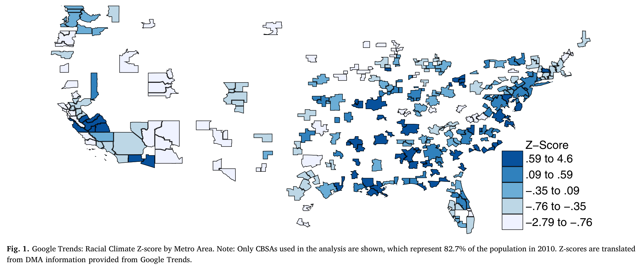
discrimination, which further influences housing decisions. To gauge the racial climate we create an average Z-score index using the following search terms/topics: Police Brutality, Black Lives Matter, Shooting of Michael Brown, Ferguson Unrest, Trayvon Martin, Death of Freddie Gray, and Shooting of Tamir Rice.<sup><a href="#source-note-11" aria-label="Source note 11">11</a></sup> Fig. 1 illustrates the average Z-scores for the racial climate in the metro areas used in the analysis.

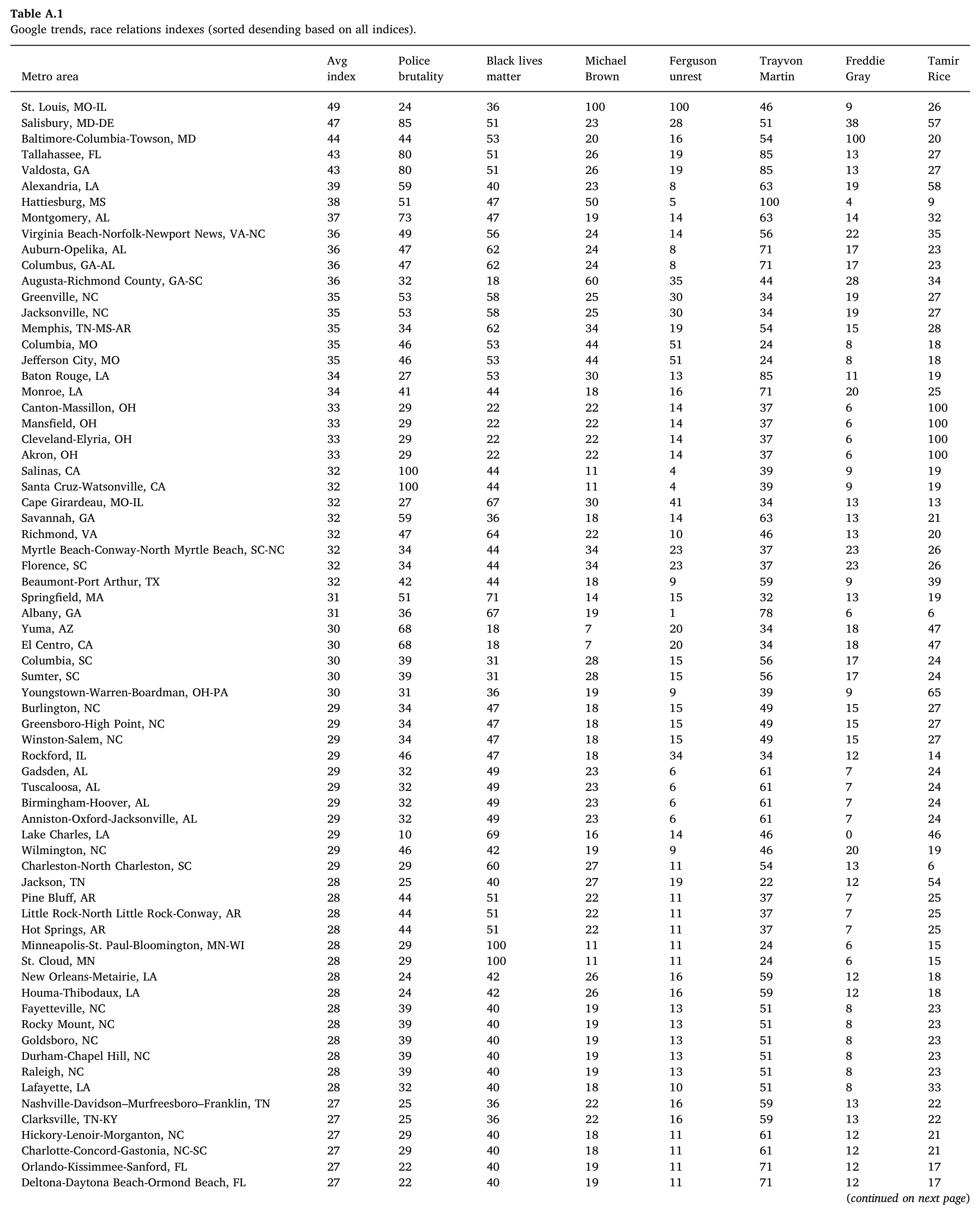
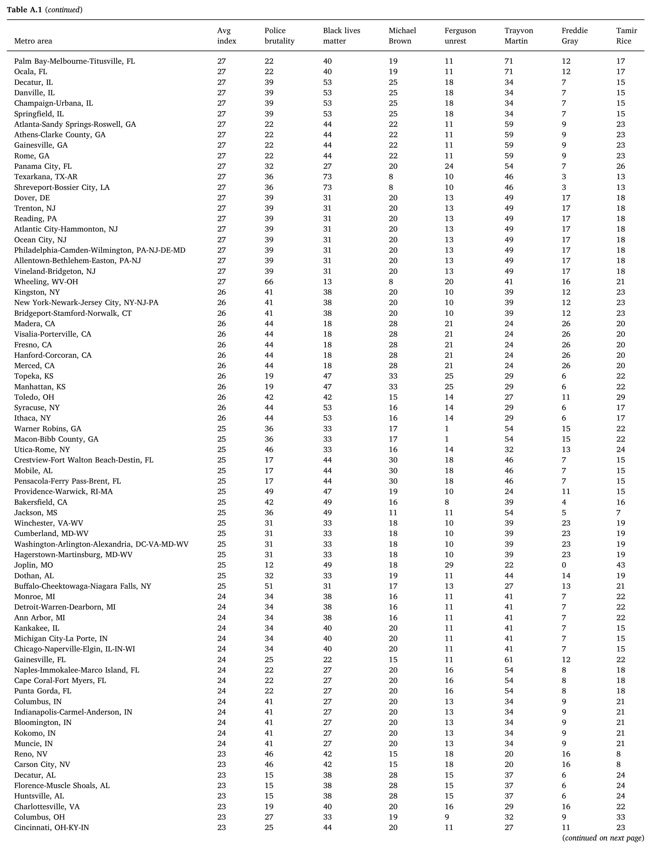
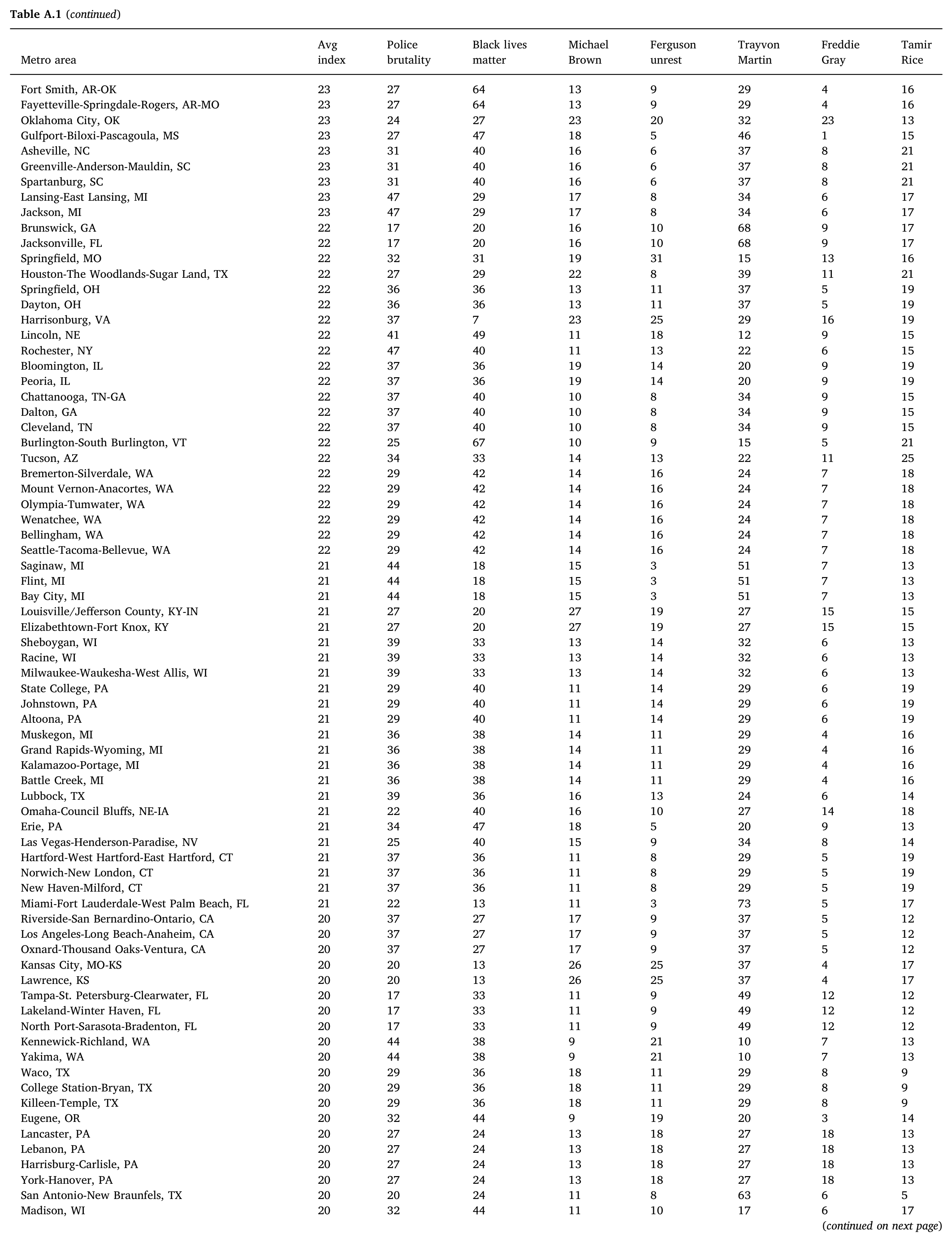
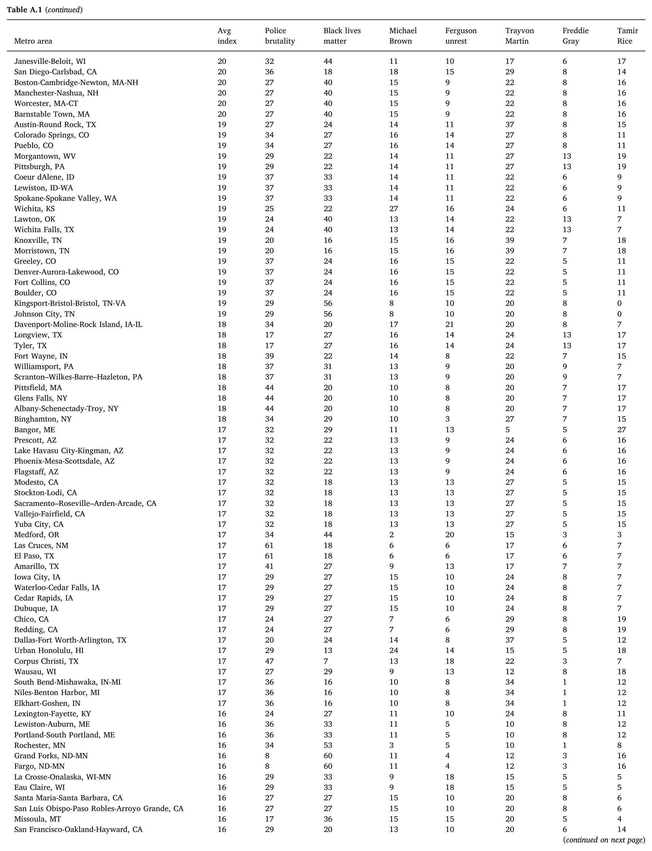
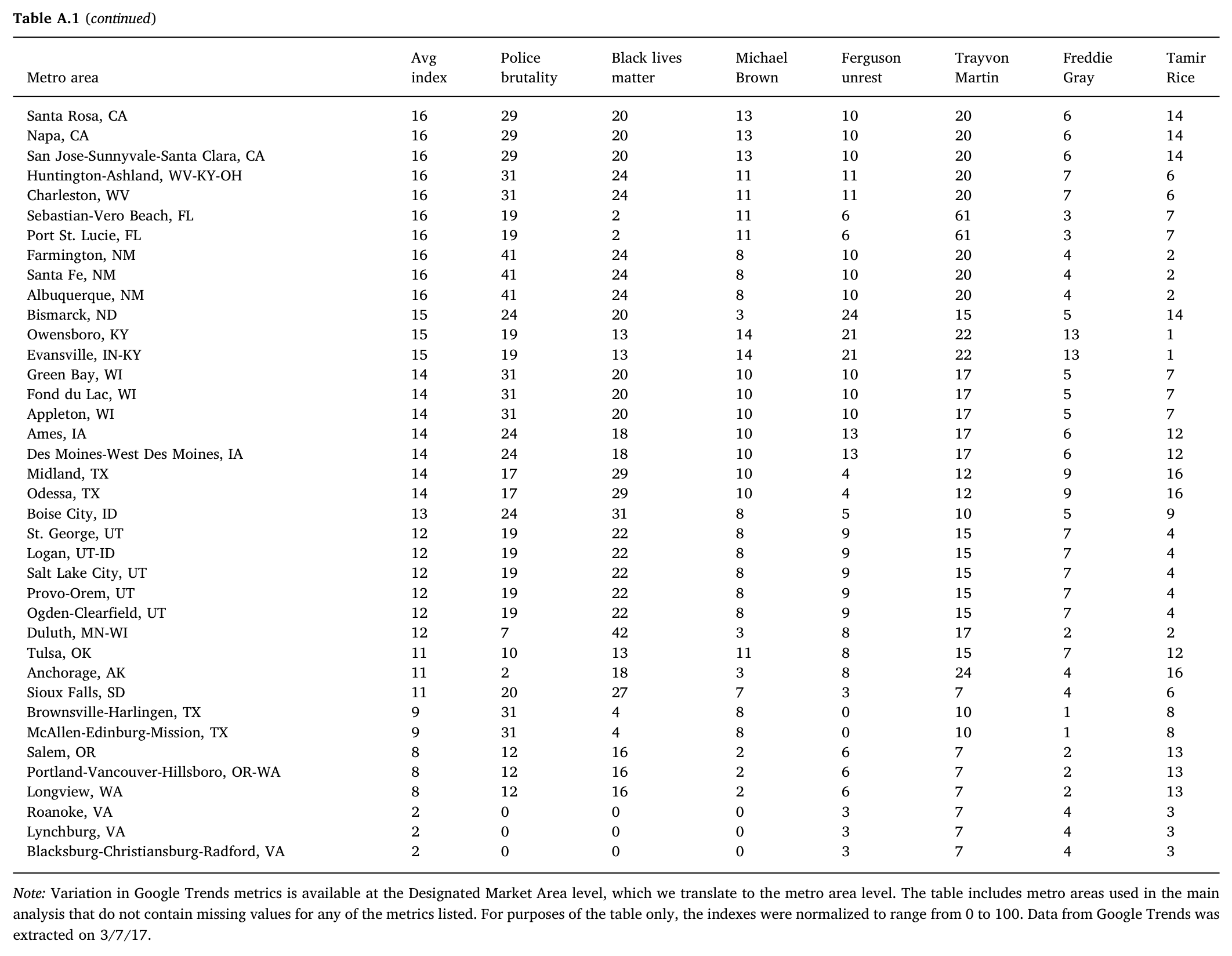
Appendix Table A.1 further illustrates the variation in the aggregate index by metro area. Several of the metro areas with the largest index for racial climate are from areas where the incidents occurred. Arguably, the incidents occurred in these metro areas because of heightened racial tensions and the flare-ups would not have necessarily occurred in different areas for the same stimulus. By aggregating search interest across several different events—that should not be correlated otherwise—we mitigate the influence of each individual event. Nonetheless, there is concern that these areas received a disproportionate amount of search interest because the incident occurred in that locality. Consequently, in a robustness check, we exclude St. Louis, Missouri; Baltimore, Maryland; Cleveland, Ohio; and Orlando,
Florida from the analysis.

The regression analysis will evaluate the relationship between racial climate and black homeownership. Anecdotally, Salem, Oregon, and Jacksonville, North Carolina provide an example of a negative relationship between racial climate and homeownership. Oregon with one of the best racial climates has a black homeownership rate of 39.7% while Jacksonville, North Carolina has one of the worst racial climates has a black homeownership rate of 32.7

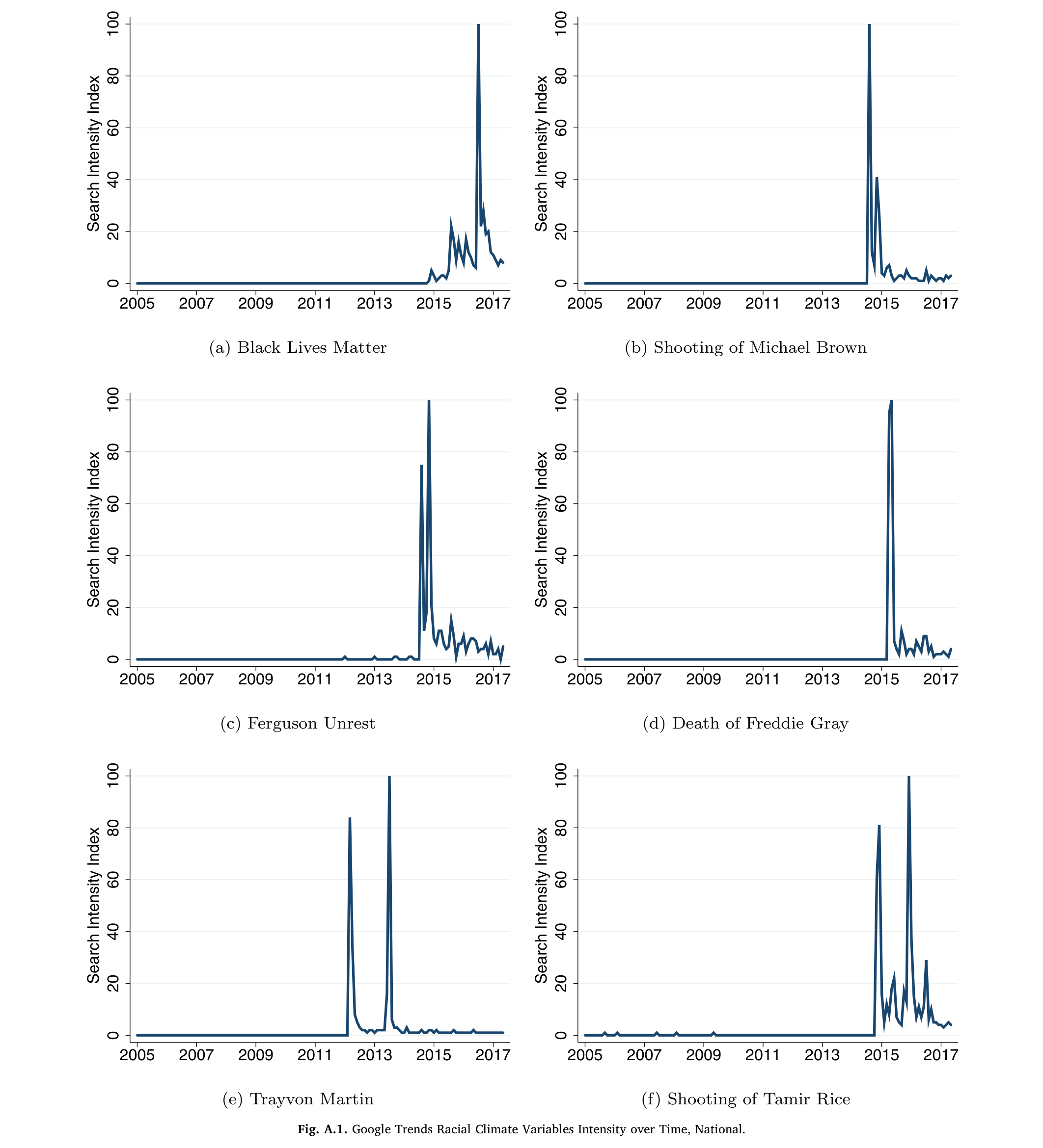
The earliest incident that we use to gauge underlying racial climate was the “Shooting of Trayvon Martin” that occurred on February 26, 2012.<sup><a href="#source-note-12" aria-label="Source note 12">12</a></sup> To disallow the event itself from driving homeownership rates (i.e., decreased black homeownership due to actual violence/destruction), we focus on a sample from the ACS that entirely predates any of the actual events, using the years 2005–2011. The racial climate metric is based on the assumption that search interest in these events is a manifestation of latent racial tension in an area rather than the event itself driving homeownership rates.

### Figure 1. Google Trends: Racial Climate Z-score by Metro Area

<figure class="article-figure" id="figure-1"><a href="/files/publications/ay-ja-nfkd4lequxehfrty-assets/figure-1.png"><img alt="Figure 1. Map of racial climate by metropolitan area, shaded in five Z-score groups from −2.79 to 4.6. The caption identifies Google Trends data and metropolitan areas covering 82.7 percent of the US population." height="896" loading="lazy" src="/files/publications/ay-ja-nfkd4lequxehfrty-assets/figure-1.png" width="2124"/></a><figcaption>Figure 1, supplied PDF page 3. <a href="/files/publications/ay-ja-nfkd4lequxehfrty-assets/figure-1.png">Open full-resolution image</a>.</figcaption></figure>

**Notes:** Only CBSAs used in the analysis are shown, which represent 82.7% of the population in 2010. Z-scores are translated from DMA information provided from Google Trends.

In addition to Google Trends data, we use other metro level data to account for factors that might influence the housing decision. These data include monthly Fair Market Rents (FMR) from the Department of Housing and Urban Development,<sup><a href="#source-note-13" aria-label="Source note 13">13</a></sup> Housing Price Index (HPI) from the Federal Housing Finance Agency (FHFA),<sup><a href="#source-note-14" aria-label="Source note 14">14</a></sup> and data from the FBI Uniform Crime Report statistics.<sup><a href="#source-note-15" aria-label="Source note 15">15</a></sup> Furthermore, we calculate the income to poverty ratio, share in manufacturing, and percent black using the ACS and the logarithm of population from the 2010 Decennial Census for each metro area.

We restrict our sample to (a) households whose head is either black or white (non-Hispanic) (b) heads who reside in metropolitan areas<sup><a href="#source-note-16" aria-label="Source note 16">16</a></sup> (c) metro areas that have information on monthly FMR from the Department of Housing and Urban Development, HPI from the Federal Housing Finance Agency, and crime statistics as reported in the FBI Uniform Crime Report. The 329 metro areas used in the analysis contain 82.7% of the U.S. population as reported in the 2010 census.

To gauge the influence of racial climate on black homeownership, we analyze three different samples of households. First, we analyze the full sample of households who reside in a metro area. However, use of the full sample raises concerns with timing of measurement and reverse causality. For our principal outcome—homeownership—it is important to recognize that the vast majority of households are established in a location and plausibly made their homeownership decision at a time in the past that reflects a different racial climate than the present climate.<sup><a href="#source-note-17" aria-label="Source note 17">17</a></sup> For example, ACS tabulations indicate that nearly 56% of all homeowners in 2011 lived in their residence for 10 or more years.

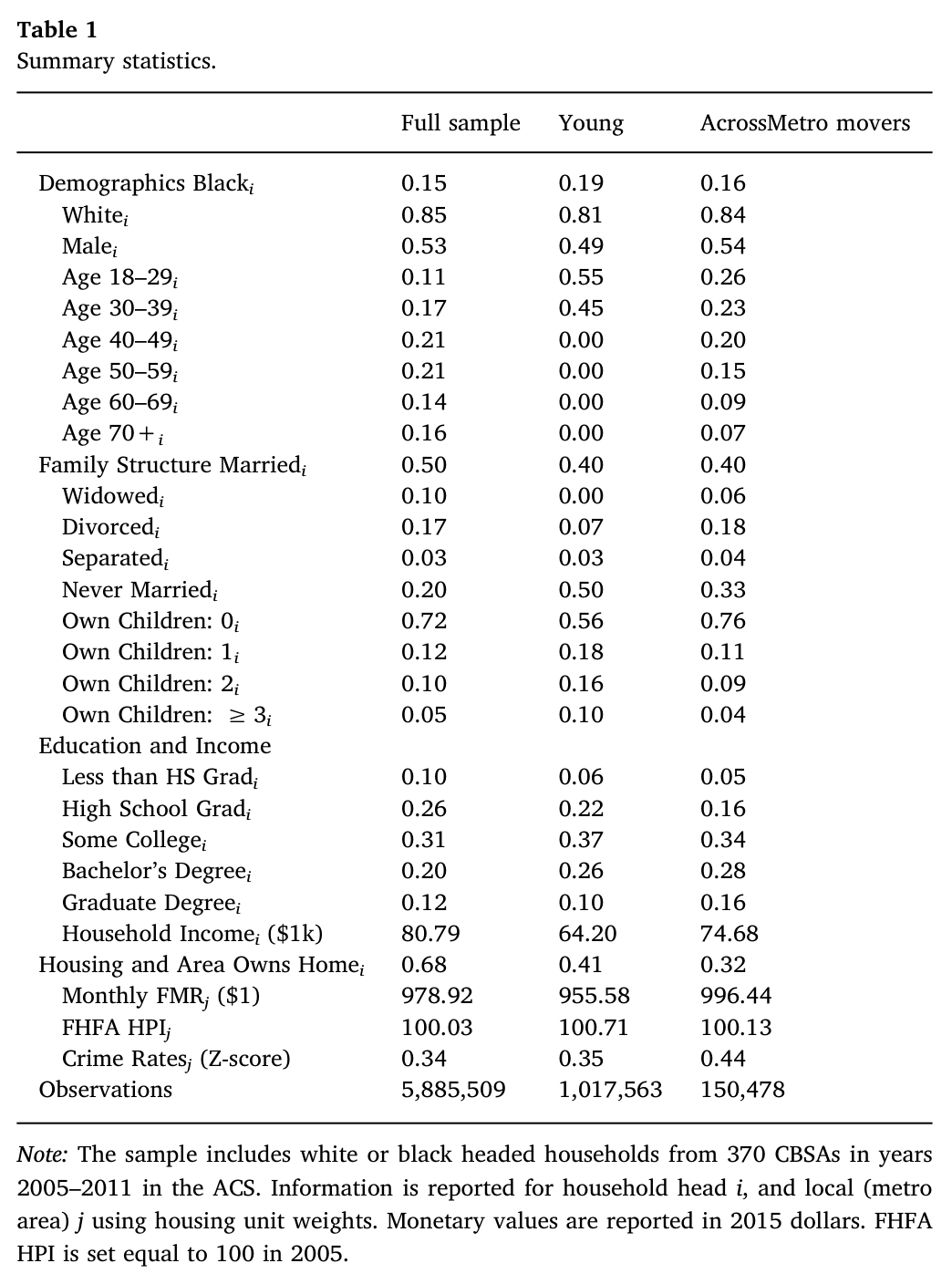
### Table 1. Summary statistics

<figure class="article-figure" id="table-1"><a href="/files/publications/ay-ja-nfkd4lequxehfrty-assets/table-1.png"><img alt="Table 1. Summary statistics for the full sample, young households and households moving between metropolitan areas: demographics, family characteristics, education, income, housing and local conditions, with sample sizes and data notes." height="1408" loading="lazy" src="/files/publications/ay-ja-nfkd4lequxehfrty-assets/table-1.png" width="1044"/></a><figcaption>Table 1, supplied PDF page 3. <a href="/files/publications/ay-ja-nfkd4lequxehfrty-assets/table-1.png">Open full-resolution image</a>.</figcaption></figure>


Therefore, the measure of racial climate derived from Google Trends data likely does not capture the characteristics of the environment that drove the rent versus own decision for a significant majority of the full sample. In addition, the homeownership rate in a metro area could influence search interest and the racial tension variable resulting in reverse causality.<sup><a href="#source-note-18" aria-label="Source note 18">18</a></sup>

As one alternative, we analyze a younger sample (household heads aged 18–35) who when surveyed likely made the homeownership decision in the recent past. For this sample, the racial climate captured by the Google Trends index variable likely better characterizes the environment when the decision to rent or own was made. Furthermore, the homeownership of the smaller sample is less likely to drive the racial climate variable mitigating concerns of reverse causality.

As another alternative, we analyze households that moved in the year prior to being surveyed. This sample includes households that actively made the decision to rent or own in the racial environment captured by the racial climate index. We exclude households that moved within a metro area as they were exposed to the same racial climate in the year prior to their move and there is persistence in the homeownership decision. Using the sample of across-metro movers also mitigates concerns for reverse causality as the small proportion of households that moved are unlikely to influence Google searches enough to significantly impact the racial climate index.

Table 1 presents the basic summary statistics for the three samples described above. As shown, the racial composition of the three samples is relatively similar with blacks representing between 15% and 19% of the sample. In relation to the full sample, the across-metro movers sample is younger, less likely to be married, better educated, and significantly less likely to own a home (32% in relative to 68%). The young sample is also less likely to be married, less likely to have children, have lower income, and are significantly less likely to own a home in comparison to the full sample.
## 3. Empirical methodology
To test for the influence of racial climate on black homeownership, we estimate the following linear probability model, in the spirit of Watson’s (2014) analysis of chilling effects of Immigration and Naturalization Service (INS) enforcement actions on non-citizens.<sup><a href="#source-note-19" aria-label="Source note 19">19</a></sup>

<figure class="article-figure" id="equation-1"><a href="/files/publications/ay-ja-nfkd4lequxehfrty-assets/equation-1.png"><img alt="Equation 1. Homeownership regression with Black household status, its interaction with racial climate, household and local characteristics, Black-by-local interactions, metropolitan and year effects, and an error term." height="132" loading="lazy" src="/files/publications/ay-ja-nfkd4lequxehfrty-assets/equation-1.png" width="1048"/></a><figcaption>Equation 1, supplied PDF page 4. <a href="/files/publications/ay-ja-nfkd4lequxehfrty-assets/equation-1.png">Open full-resolution image</a>.</figcaption></figure>

where <math xmlns="http://www.w3.org/1998/Math/MathML" display="inline"><mrow><mi>O</mi><mi>w</mi><msub><mi>n</mi><mrow><mi>i</mi><mi>j</mi><mi>t</mi></mrow></msub></mrow></math> is an indicator that household i owned a home in location j at time t rather than rent and <math xmlns="http://www.w3.org/1998/Math/MathML" display="inline"><mrow><mi>B</mi><mi>l</mi><mi>a</mi><mi>c</mi><msub><mi>k</mi><mi>i</mi></msub></mrow></math> is an indicator that the head of the household is black. <math xmlns="http://www.w3.org/1998/Math/MathML" display="inline"><mrow><mi>C</mi><mi>l</mi><mi>i</mi><mi>m</mi><mi>a</mi><mi>t</mi><msub><mi>e</mi><mi>j</mi></msub></mrow></math> is the time-invariant index for the racial climate that varies at the DMA level (higher values represent a worse racial climate). Xi measures characteristics of the head and other family members including age, gender, marital status, educational attainment, and number of children. <math xmlns="http://www.w3.org/1998/Math/MathML" display="inline"><mrow><mi>L</mi><mi>o</mi><mi>c</mi><mi>a</mi><msub><mi>l</mi><mrow><mi>j</mi><mi>t</mi></mrow></msub></mrow></math> measures factors that vary across cities and over time including FMR, HPI, Crime Rates, and percent in manufacturing.<sup><a href="#source-note-20" aria-label="Source note 20">20</a></sup> Following Cutler and Glaeser (1997) we also include the interaction <math xmlns="http://www.w3.org/1998/Math/MathML" display="inline"><mrow><mi>B</mi><mi>l</mi><mi>a</mi><mi>c</mi><msub><mi>k</mi><mi>i</mi></msub></mrow></math> × <math xmlns="http://www.w3.org/1998/Math/MathML" display="inline"><mrow><mi>L</mi><mi>o</mi><mi>c</mi><mi>a</mi><msub><mi>l</mi><mrow><mi>j</mi><mi>t</mi></mrow></msub></mrow></math> to allow for differential location effects on blacks relative to whites. In addition, we include the interaction of race with other locality characteristics including logarithm of the population in 2010, income to poverty ratio, and percent black. <math xmlns="http://www.w3.org/1998/Math/MathML" display="inline"><mrow><msub><mi>&#x003B4;</mi><mi>j</mi></msub></mrow></math> and <math xmlns="http://www.w3.org/1998/Math/MathML" display="inline"><mrow><msub><mi>&#x003B4;</mi><mi>t</mi></msub></mrow></math> are fixed effects for locality and time. The specification does not include <math xmlns="http://www.w3.org/1998/Math/MathML" display="inline"><mrow><mi>C</mi><mi>l</mi><mi>i</mi><mi>m</mi><mi>a</mi><mi>t</mi><msub><mi>e</mi><mi>j</mi></msub></mrow></math> itself since it is subsumed with locality fixed effects. The locality fixed effects control for differences in levels for home prices, whereas the HPI controls for differences in growth of housing prices over time. Locality fixed effects also control for time invariant racial differences in the residential location inside a metro area, which influence homeownership rates (Deng et al., 2003). The error term <math xmlns="http://www.w3.org/1998/Math/MathML" display="inline"><mrow><msub><mi>&#x003B5;</mi><mrow><mi>i</mi><mi>j</mi><mi>t</mi></mrow></msub></mrow></math> is corrected for clustering at the DMA level.

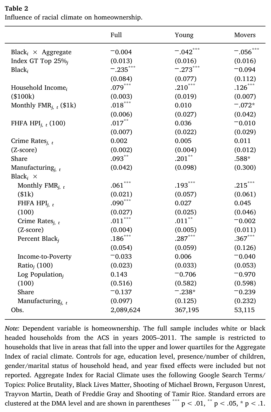
### Table 2. Influence of racial climate on homeownership

<figure class="article-figure" id="table-2"><a href="/files/publications/ay-ja-nfkd4lequxehfrty-assets/table-2.png"><img alt="Table 2. Estimated association between racial climate and homeownership for the full sample, young households and households moving between metropolitan areas; coefficient estimates, standard errors, observation counts and model notes." height="1588" loading="lazy" src="/files/publications/ay-ja-nfkd4lequxehfrty-assets/table-2.png" width="1044"/></a><figcaption>Table 2, supplied PDF page 4. <a href="/files/publications/ay-ja-nfkd4lequxehfrty-assets/table-2.png">Open full-resolution image</a>.</figcaption></figure>


Under the assumption that higher values of <math xmlns="http://www.w3.org/1998/Math/MathML" display="inline"><mrow><mi>C</mi><mi>l</mi><mi>i</mi><mi>m</mi><mi>a</mi><mi>t</mi><msub><mi>e</mi><mi>j</mi></msub></mrow></math> reflect a worse racial climate, we expect the coefficient <math xmlns="http://www.w3.org/1998/Math/MathML" display="inline"><mrow><msub><mi>&#x003B2;</mi><mn>1</mn></msub></mrow></math>—the interaction of a worse racial climate and black—to be negative. The coefficient captures at least two effects. First, black households may choose not to invest in a community with a poor racial climate and decide to rent instead. Second, households may select a location based on the racial climate. If this selection occurs, homeownership rates in communities with a good racial climate will be higher while simultaneously reducing the homeownership rate in communities with a poor racial climate.<sup><a href="#source-note-21" aria-label="Source note 21">21</a></sup> Therefore, <math xmlns="http://www.w3.org/1998/Math/MathML" display="inline"><mrow><msub><mi>&#x003B2;</mi><mn>1</mn></msub></mrow></math> can be interpreted as capturing the net effect of these two behaviors (which work in the same direction). Identification comes from the
assumption that the racial climate does not affect the investment/ownership decision of white households; therefore, our specification nets out other fixed local characteristics with <math xmlns="http://www.w3.org/1998/Math/MathML" display="inline"><mrow><msub><mi>&#x003B4;</mi><mi>j</mi></msub></mrow></math>. In addition to the selection of location, there is also selection in the decision to relocate. The estimate will not capture this effect, which could lead to an underestimation of the influence on racial climate on black homeownership.


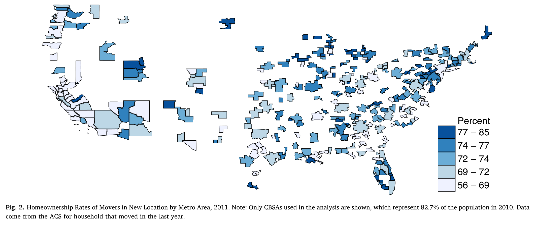
### Figure 2

<figure class="article-figure" id="figure-2"><a href="/files/publications/ay-ja-nfkd4lequxehfrty-assets/figure-2.png"><img alt="Figure 2. Map of 2011 homeownership rates among households that moved to a new metropolitan area, with five percentage groups spanning 56 to 85 percent and an American Community Survey source note." height="896" loading="lazy" src="/files/publications/ay-ja-nfkd4lequxehfrty-assets/figure-2.png" width="2124"/></a><figcaption>Figure 2, supplied PDF page 5. <a href="/files/publications/ay-ja-nfkd4lequxehfrty-assets/figure-2.png">Open full-resolution image</a>.</figcaption></figure>

### Figure 3

<figure class="article-figure" id="figure-3"><a href="/files/publications/ay-ja-nfkd4lequxehfrty-assets/figure-3.png"><img alt="Figure 3. Distribution of predicted homeownership in movers’ former locations, on a zero-to-one horizontal scale. Arrows identify the Bronx near 0.33 and Nashville near 0.78; the accompanying note explains demographic matching." height="868" loading="lazy" src="/files/publications/ay-ja-nfkd4lequxehfrty-assets/figure-3.png" width="2124"/></a><figcaption>Figure 3, supplied PDF page 5. <a href="/files/publications/ay-ja-nfkd4lequxehfrty-assets/figure-3.png">Open full-resolution image</a>.</figcaption></figure>

## 4. Results
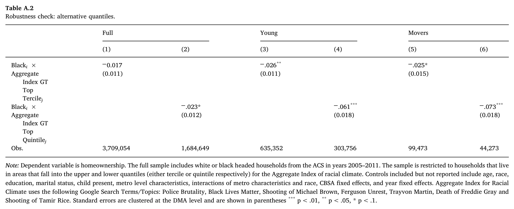
Table 2 presents the results from our analysis of the three main samples. The main variable is a control for residing in an area with a racial climate index in the highest quartile. We drop observations in the middle quartiles such that the comparison is between the top and bottom quartiles.<sup><a href="#source-note-22" aria-label="Source note 22">22</a></sup>

The first column shows no evidence that the racial climate negatively impacts either race’s homeownership decision. Nonetheless, as outlined, the full specification analyzes the influence of the current racial climate on homeownership for individuals that made the decision under a presumably different climate and also is subject to concerns of reverse causality.

In the second column, we repeat the analysis for households headed by individuals aged 18–35 who likely made the homeownership decision under the racial climate captured by the racial climate index. The results indicate that black households in the most racially charged
metro areas are 4.2 percentage points (p-value < .001) less likely to purchase a home relative to those in the least racially charged areas from a base of 25.0% black homeownership. The last column of Table 2 presents the results from the sample of across-metro movers. The results indicate that black households in the most racially charged metro areas are 5.6 percentage points less likely to purchase a home (from a base of 20.3% black homeownership).<sup><a href="#source-note-23" aria-label="Source note 23">23</a></sup> Across the specifications, blacks are significantly less likely to be homeowners. Blacks are more likely to purchase a home relative to whites as FMR or the HPI increases. Higher crime rates are correlated with increased black homeownership while largely uncorrelated with white homeownership. The proportion of black households in a metro area is also associated with increased black homeownership. Although not presented in the table, the results are consistent with the standard findings that ownership rises with age, education level, marriage and presence of children.

### Table 3. Influence of previous homeownership

<figure class="article-figure" id="table-3"><a href="/files/publications/ay-ja-nfkd4lequxehfrty-assets/table-3.png"><img alt="Table 3. Four homeownership regressions adding measures of likely ownership in the former location, with the Black-by-racial-climate coefficient, demographic matching definitions, standard errors and sample notes." height="720" loading="lazy" src="/files/publications/ay-ja-nfkd4lequxehfrty-assets/table-3.png" width="1044"/></a><figcaption>Table 3, supplied PDF page 5. <a href="/files/publications/ay-ja-nfkd4lequxehfrty-assets/table-3.png">Open full-resolution image</a>.</figcaption></figure>


### Table 4. Influence of racial climate on homeownership, robustness checks

<figure class="article-figure" id="table-4"><a href="/files/publications/ay-ja-nfkd4lequxehfrty-assets/table-4.png"><img alt="Table 4. Racial-climate robustness checks excluding hot spots, controlling for climate-change searches, former racial climate or segregation, and separating 2005–2008 from 2009–2011; estimates, standard errors, sample sizes and notes." height="728" loading="lazy" src="/files/publications/ay-ja-nfkd4lequxehfrty-assets/table-4.png" width="2124"/></a><figcaption>Table 4, supplied PDF page 6. <a href="/files/publications/ay-ja-nfkd4lequxehfrty-assets/table-4.png">Open full-resolution image</a>.</figcaption></figure>


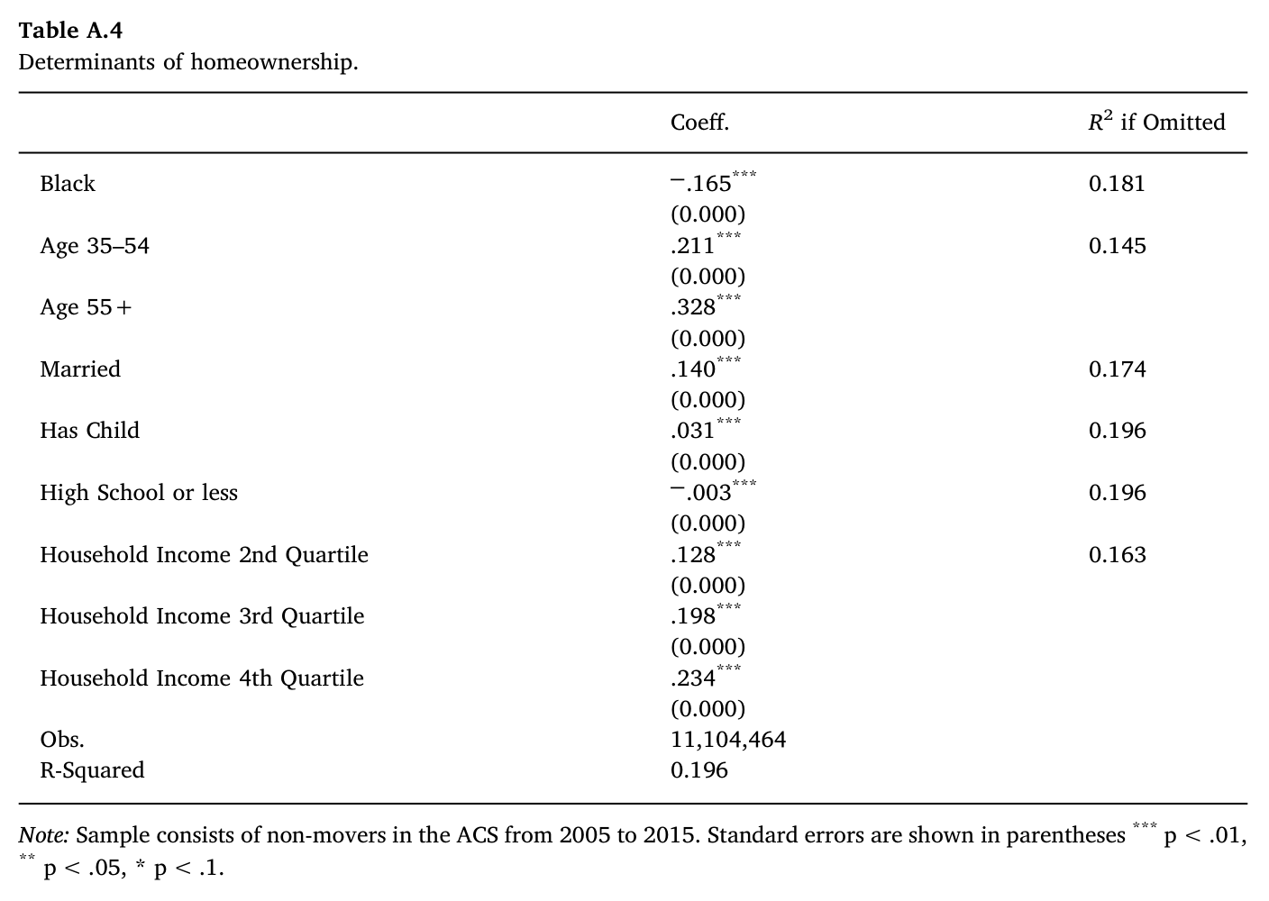
A important consideration for the across-metro movers sample is the persistence in homeownership across moves due to preferences and home equity. Although the ACS does not contain information on the previous homeownership status of movers, it does contain information on the household’s original location. To account for differences in the likelihood that a household owned a home, we construct a measure of the average homeownership rate of non-movers in the location from which the household moved with similar characteristics. In constructing the measure, there is a trade-off of including many characteristics and having a precise match with small cell sizes or including a few characteristics but having large cell sizes. To determine which characteristics to use in the creation of
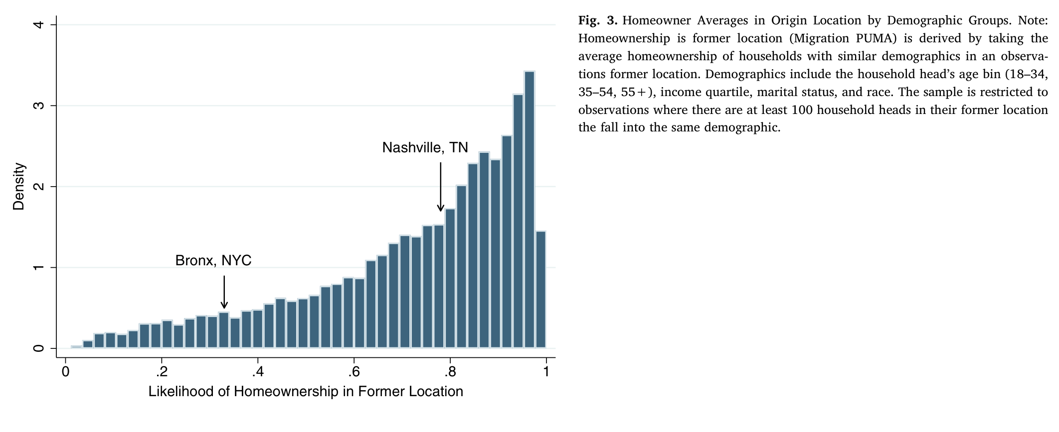
the metric, we first estimate a simple model of homeownership on standard demographic controls.<sup><a href="#source-note-24" aria-label="Source note 24">24</a></sup> To rank order the controls, we run the full model and obtain the R<sup>2</sup> and then run the model repeatedly leaving out individual variables (or groups of variables) one at a time noting the R<sup>2</sup> for each model. Based on the difference in explained variation in homeownership, we determine that the most influential variables are age and income. We construct the first measure using these two characteristics. We then create two more measures using progressively more of the demographics based on importance in explaining homeownership.<sup><a href="#source-note-25" aria-label="Source note 25">25</a></sup> Fig. 3 shows the distribution of homeownership for non-movers based on demographic group and location using the second
measure containing age, income, marital status, and race. As an example, the likelihood of
homeownership in the previous location for household heads aged between 35 and 54, with income between $30,000 and $60,000, were married, and white was 31% in the Bronx of New York City and 78% in Nashville, Tennessee.

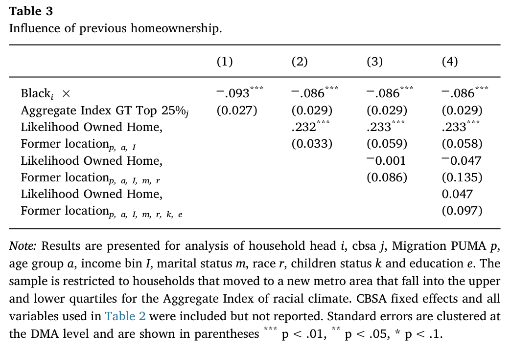
Table 3 analyzes the sensitivity of the results to controlling for the likelihood of homeownership prior to the move. The first column replicates the results from the across-metro movers presented in Table 2 but with the restricted sample originating from the exclusion of observations where there were insufficient data to estimate the likelihood of homeownership for a particular location and demographic cell. The last three columns sequentially add controls for the likelihood of homeownership keeping sample sizes constant for comparison. The estimates are extremely stable with the inclusion of additional controls indicating that our racial climate results are unlikely to be driven by omitted variable bias related to previous homeownership. Among across-metro movers, a charged racial climate reduces black homeownership by 9 percentage
points controlling for the likelihood of previous homeownership.
## 5. Robustness
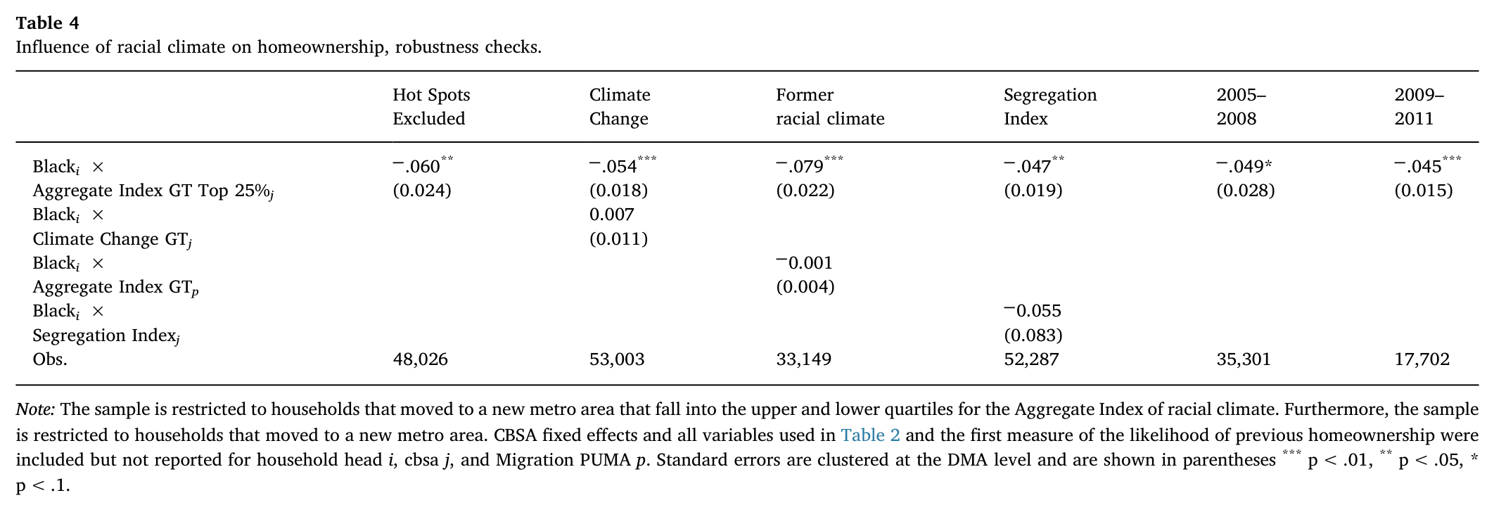
Table 4 contains the results from several different robustness checks using the across-metro movers sample with locality fixed effects and interactions of race and metro characteristics as the baseline model.<sup><a href="#source-note-26" aria-label="Source note 26">26</a></sup> The first column excludes observations from the focal points of the events that were used in the derivation of our index of racial climate. In particular, we exclude the four “hot spots” of St. Louis, Missouri; Baltimore, Maryland; Cleveland, Ohio; and Orlando, Florida. This exclusion address concerns that search intensity in the area of the actual event might be elevated given the location rather than representing heightened racial tensions. As shown, the magnitudes are not sensitive to the exclusion of these areas; even excluding these areas, black homeownership falls by 6 percentage
points.

A possible concern with the metric used to measure racial climate is that it might be correlated with other forms of social activism. In the second column, we add an interaction between the Z-score for Google searches of “Climate Change” and <math xmlns="http://www.w3.org/1998/Math/MathML" display="inline"><mrow><mi>B</mi><mi>l</mi><mi>a</mi><mi>c</mi><msub><mi>k</mi><mi>i</mi></msub></mrow></math> to control for possible correlations between social activism and search interest in incidents related to racial climate. The results are nearly identical to the main specification that excludes the interaction for climate change. This indicates that our metric of racial climate is unlikely to be driven by social activism rather than increased racial tensions.

In the third column, we present results from a specification that account for the racial climate in the former location. Previous racial climate presumably influenced the homeownership decision. Through persistence in homeownership, the former racial climate could impact homeownership in the new location and consequently bias the results. The point estimate for the specification increases in absolute magnitude but the difference is driven by the sample and not the inclusion of the added control.<sup><a href="#source-note-27" aria-label="Source note 27">27</a></sup> Furthermore, as in the full sample of households, the timing of the measurement for the previous racial climate’s homeownership decision likely will not reflect the racial climate when they made the decision to rent or buy a home in the previous location.

### Table 5. Sensitivity to events used in index, leave-one-out

<figure class="article-figure" id="table-5"><a href="/files/publications/ay-ja-nfkd4lequxehfrty-assets/table-5.png"><img alt="Table 5. Leave-one-out sensitivity of the racial-climate index, separately excluding police brutality, Black Lives Matter, Ferguson/Michael Brown, Trayvon Martin, Freddie Gray and Tamir Rice; estimates, standard errors and observations." height="860" loading="lazy" src="/files/publications/ay-ja-nfkd4lequxehfrty-assets/table-5.png" width="2124"/></a><figcaption>Table 5, supplied PDF page 7. <a href="/files/publications/ay-ja-nfkd4lequxehfrty-assets/table-5.png">Open full-resolution image</a>.</figcaption></figure>


Another potential concern in that the racial climate index could be picking up the influence of other features of an urban area such as racial segregation that differentially impact black households. To control for differences in racial composition/segregation within metro areas, we construct a dissimilarities index following Cutler and Glaeser (1997). We use 2010 Decennial Census data with racial counts at the census tract level, which proxies for neighborhoods.<sup><a href="#source-note-28" aria-label="Source note 28">28</a></sup> Housing segregation in a metro area is defined as:

<figure class="article-figure" id="equation-2"><a href="/files/publications/ay-ja-nfkd4lequxehfrty-assets/equation-2.png"><img alt="Equation 2. Housing segregation equals one half of the sum, over areas, of the absolute difference between each area’s share of the Black population and its share of the White population." height="144" loading="lazy" src="/files/publications/ay-ja-nfkd4lequxehfrty-assets/equation-2.png" width="1048"/></a><figcaption>Equation 2, supplied PDF page 7. <a href="/files/publications/ay-ja-nfkd4lequxehfrty-assets/equation-2.png">Open full-resolution image</a>.</figcaption></figure>


where <math xmlns="http://www.w3.org/1998/Math/MathML" display="inline"><mrow><mi>B</mi><mi>l</mi><mi>a</mi><mi>c</mi><msub><mi>k</mi><mi>i</mi></msub></mrow></math> (<math xmlns="http://www.w3.org/1998/Math/MathML" display="inline"><mrow><mi>W</mi><mi>h</mi><mi>i</mi><mi>t</mi><msub><mi>e</mi><mi>i</mi></msub></mrow></math>) is the number of blacks (whites) in census tract i and Black (White) is the number of blacks (whites) in the metro area. If blacks are evening distributed across the metro area, then the index would be zero. If there is complete segregation, then the index would be one. As reported in Table 4, the inclusion of this measure interacted with race does not alter the main finding and the interacted measure itself is not statistically significant. This finding indicates that racial segregation does not differentially impact blacks’ rent versus own decision relative to whites.

As we are using search interest in very contemporaneous events the racial climate might be different for the earliest years of our sample. To test for this possibility, we split the sample between the earlier years (2005–2008) and the years directly preceding the Black Lives Matter movements (2009–2011). The last two columns of Table 4 present the results and once again there is a consistent negative relationship between the likelihood of homeownership for blacks and a poor racial climate. The results, however, are weakly statistically significant in the earlier sample but strongly statistically significant in the later sample.

These findings provide greater support for looking at households in transition (movers) rather than the full sample as the racial climate or the impact of racial climate appears to change over time.

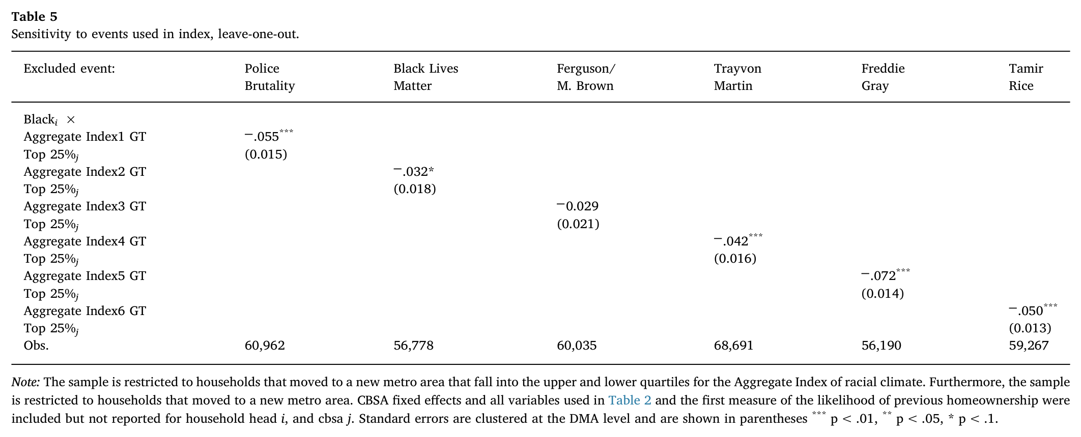
Lastly, we analyze the importance of the events included in the construction of the racial climate index. We run the main specification of movers repeatedly excluding one of the search topics from the construction of the index (leave-one-out approach) to analyze the influence on the main result. Table 5 presents the findings. There is still a significant impact of the racial climate on black homeownership in five out of six specifications, however, for the exclusion of the events surrounding Ferguson Missouri the coefficient becomes statistically insignificant. These results highlight some variability in the magnitude of the effect of racial climate depending on the inputs into the racial climate variable.
## 6. Conclusion
Innovations in creating data and measuring sentiment—via Google Trends—has opened up new possibilities for examining important issues, such as the role for chilling effects on behavior. The costly decision to own—and subsequently invest more in a community—is likely related to the community’s amenities and disamenities. We show that negative race relations—as represented by public interest in well publicized policing incidents—significantly reduces minority home ownership in a community. The results vary by specification, but our preferred specification shows that blacks in the most charged racial climate purchase homes 5.6 percentage points less than those who reside in localities with the least charged racial climate from a base of 20.3% black homeownership. Not only does this imply that
these households are not receiving the benefits of homeownership, but it also implies that black households are less likely to invest in their communities. (Fig. 2)
Our results, insofar as they capture problems with the criminal justice system, suggest that some recent proposals with bipartisan support to reform policing and sentencing may have larger social benefits beyond those directly aggrieved. Reforms in police tactics—such as additional training, body cameras, and the use of outside agencies to investigate misconduct—have broad-based support (Ekins, 2016). The results suggest that efforts to reform police conduct could have the positive spillover of greater community investment. Furthermore, inasmuch as homeownership increases wealth accumulation, these policy reforms could help mitigate the overall racial wealth gap.


## Appendix A
### Table A1. Google trends, race relations indexes (sorted desending based on all indices)

<figure class="article-figure" id="table-a1-page-8"><a href="/files/publications/ay-ja-nfkd4lequxehfrty-assets/table-a1-page-8.png"><img alt="Table A1, panel 1 of 5. Metropolitan racial-climate indices from St. Louis, Missouri–Illinois through Deltona–Daytona Beach–Ormond Beach, Florida, with the average index and seven Google Trends search-topic indices, sorted by the average index." height="2644" loading="lazy" src="/files/publications/ay-ja-nfkd4lequxehfrty-assets/table-a1-page-8.png" width="2124"/></a><figcaption>Table A1, supplied PDF page 8. <a href="/files/publications/ay-ja-nfkd4lequxehfrty-assets/table-a1-page-8.png">Open full-resolution image</a>.</figcaption></figure>
<figure class="article-figure" id="table-a1-page-9"><a href="/files/publications/ay-ja-nfkd4lequxehfrty-assets/table-a1-page-9.png"><img alt="Table A1, panel 2 of 5. Metropolitan racial-climate indices from Palm Bay–Melbourne–Titusville, Florida through Cincinnati, Ohio–Kentucky–Indiana, with the average index and seven Google Trends search-topic indices, sorted by the average index." height="2772" loading="lazy" src="/files/publications/ay-ja-nfkd4lequxehfrty-assets/table-a1-page-9.png" width="2124"/></a><figcaption>Table A1 (continued), supplied PDF page 9. <a href="/files/publications/ay-ja-nfkd4lequxehfrty-assets/table-a1-page-9.png">Open full-resolution image</a>.</figcaption></figure>
<figure class="article-figure" id="table-a1-page-10"><a href="/files/publications/ay-ja-nfkd4lequxehfrty-assets/table-a1-page-10.png"><img alt="Table A1, panel 3 of 5. Metropolitan racial-climate indices from Fort Smith, Arkansas–Oklahoma through Madison, Wisconsin, with the average index and seven Google Trends search-topic indices, sorted by the average index." height="2772" loading="lazy" src="/files/publications/ay-ja-nfkd4lequxehfrty-assets/table-a1-page-10.png" width="2124"/></a><figcaption>Table A1 (continued), supplied PDF page 10. <a href="/files/publications/ay-ja-nfkd4lequxehfrty-assets/table-a1-page-10.png">Open full-resolution image</a>.</figcaption></figure>
<figure class="article-figure" id="table-a1-page-11"><a href="/files/publications/ay-ja-nfkd4lequxehfrty-assets/table-a1-page-11.png"><img alt="Table A1, panel 4 of 5. Metropolitan racial-climate indices from Janesville–Beloit, Wisconsin through San Francisco–Oakland–Hayward, California, with the average index and seven Google Trends search-topic indices, sorted by the average index." height="2772" loading="lazy" src="/files/publications/ay-ja-nfkd4lequxehfrty-assets/table-a1-page-11.png" width="2124"/></a><figcaption>Table A1 (continued), supplied PDF page 11. <a href="/files/publications/ay-ja-nfkd4lequxehfrty-assets/table-a1-page-11.png">Open full-resolution image</a>.</figcaption></figure>
<figure class="article-figure" id="table-a1-page-12"><a href="/files/publications/ay-ja-nfkd4lequxehfrty-assets/table-a1-page-12.png"><img alt="Table A1, panel 5 of 5. Metropolitan racial-climate indices from Santa Rosa, California through Blacksburg–Christiansburg–Radford, Virginia, with the average index and seven Google Trends search-topic indices, sorted by the average index. The final note explains 0-to-100 normalization and the March 7, 2017 extraction date." height="1648" loading="lazy" src="/files/publications/ay-ja-nfkd4lequxehfrty-assets/table-a1-page-12.png" width="2124"/></a><figcaption>Table A1 (continued), supplied PDF page 12. <a href="/files/publications/ay-ja-nfkd4lequxehfrty-assets/table-a1-page-12.png">Open full-resolution image</a>.</figcaption></figure>


### Table A2. Robustness check: alternative quantiles

<figure class="article-figure" id="table-a2"><a href="/files/publications/ay-ja-nfkd4lequxehfrty-assets/table-a2.png"><img alt="Table A2. Robustness checks using upper and lower terciles or quintiles of the racial-climate index for full, young and mover samples, with interaction coefficients, standard errors, sample sizes and model notes." height="864" loading="lazy" src="/files/publications/ay-ja-nfkd4lequxehfrty-assets/table-a2.png" width="2124"/></a><figcaption>Table A2, supplied PDF page 12. <a href="/files/publications/ay-ja-nfkd4lequxehfrty-assets/table-a2.png">Open full-resolution image</a>.</figcaption></figure>


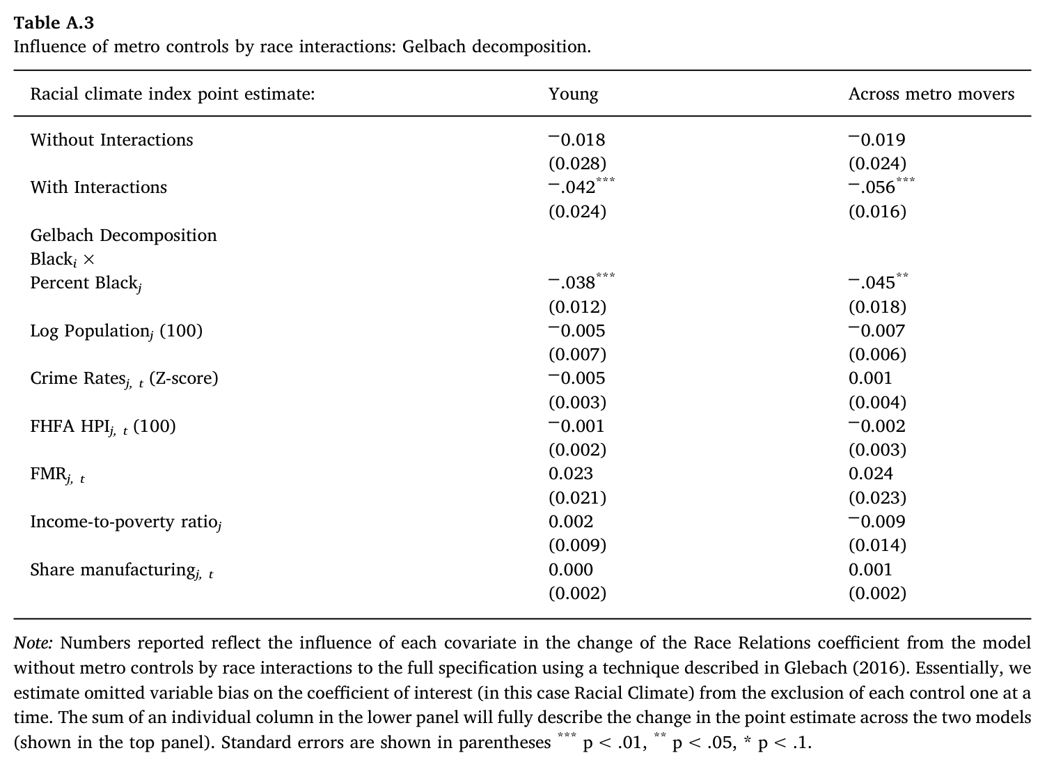
### Table A3. Influence of metro controls by race interactions: Gelbach decomposition

<figure class="article-figure" id="table-a3"><a href="/files/publications/ay-ja-nfkd4lequxehfrty-assets/table-a3.png"><img alt="Table A3. Gelbach decomposition of changes in the racial-climate coefficient after adding metro characteristics interacted with race, for young households and movers. Rows cover population, race share, crime, house prices, rent, poverty and manufacturing." height="1104" loading="lazy" src="/files/publications/ay-ja-nfkd4lequxehfrty-assets/table-a3.png" width="1504"/></a><figcaption>Table A3, supplied PDF page 13. <a href="/files/publications/ay-ja-nfkd4lequxehfrty-assets/table-a3.png">Open full-resolution image</a>.</figcaption></figure>


### Table A4. Determinants of homeownership

<figure class="article-figure" id="table-a4"><a href="/files/publications/ay-ja-nfkd4lequxehfrty-assets/table-a4.png"><img alt="Table A4. Homeownership regressions among non-movers: coefficients for race, age, marriage, children, education and income, with R-squared when characteristics are omitted, total observations and standard errors." height="1000" loading="lazy" src="/files/publications/ay-ja-nfkd4lequxehfrty-assets/table-a4.png" width="1408"/></a><figcaption>Table A4, supplied PDF page 13. <a href="/files/publications/ay-ja-nfkd4lequxehfrty-assets/table-a4.png">Open full-resolution image</a>.</figcaption></figure>


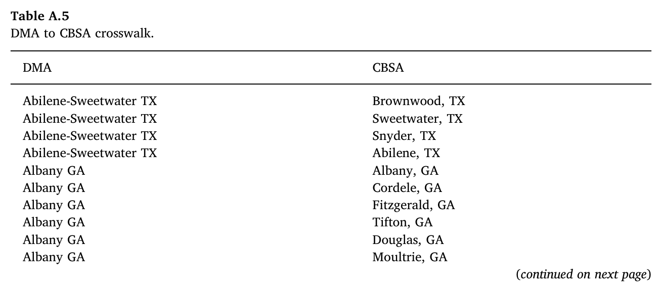
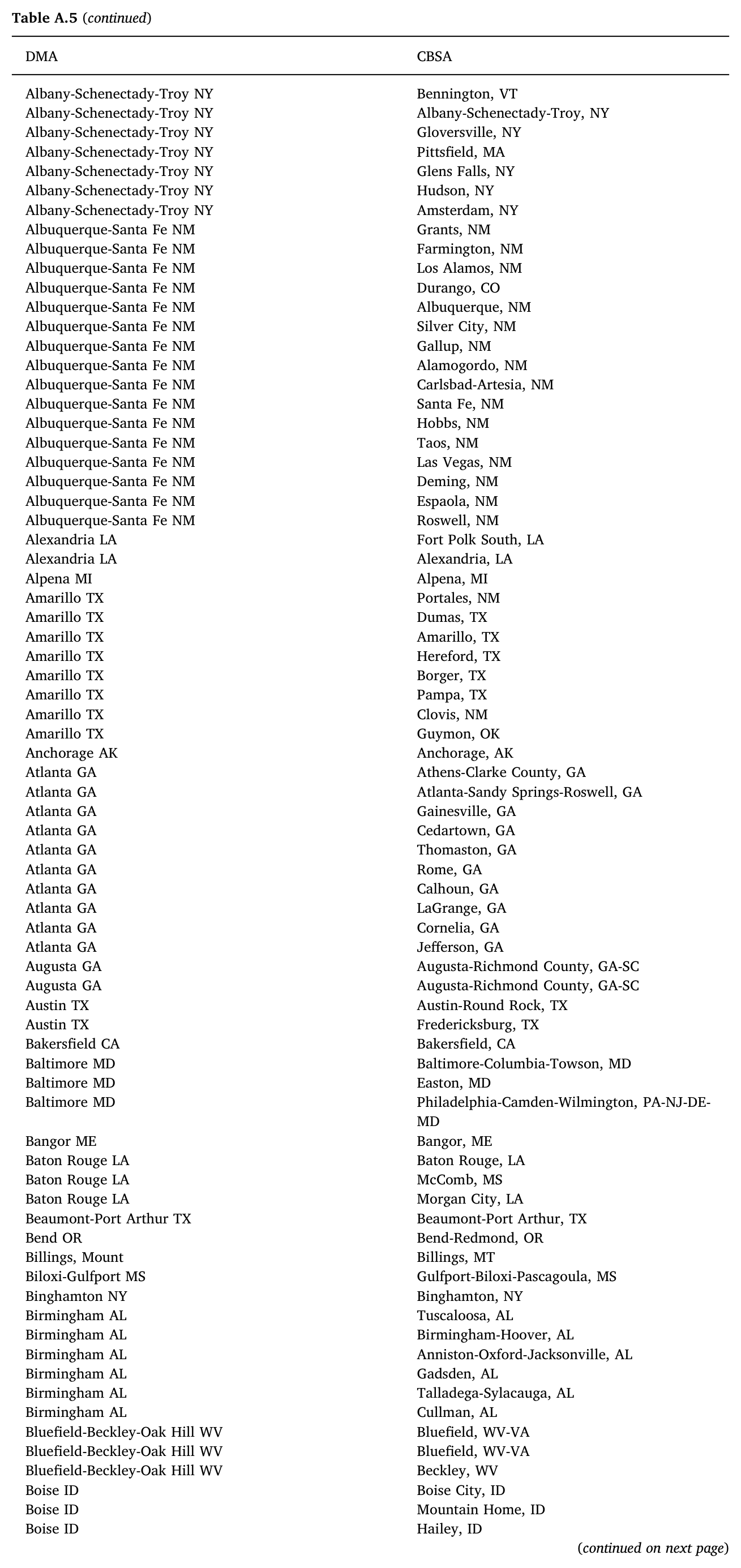
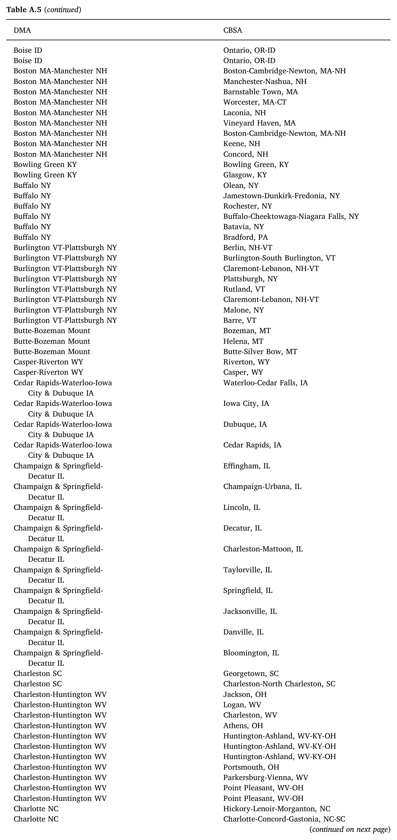
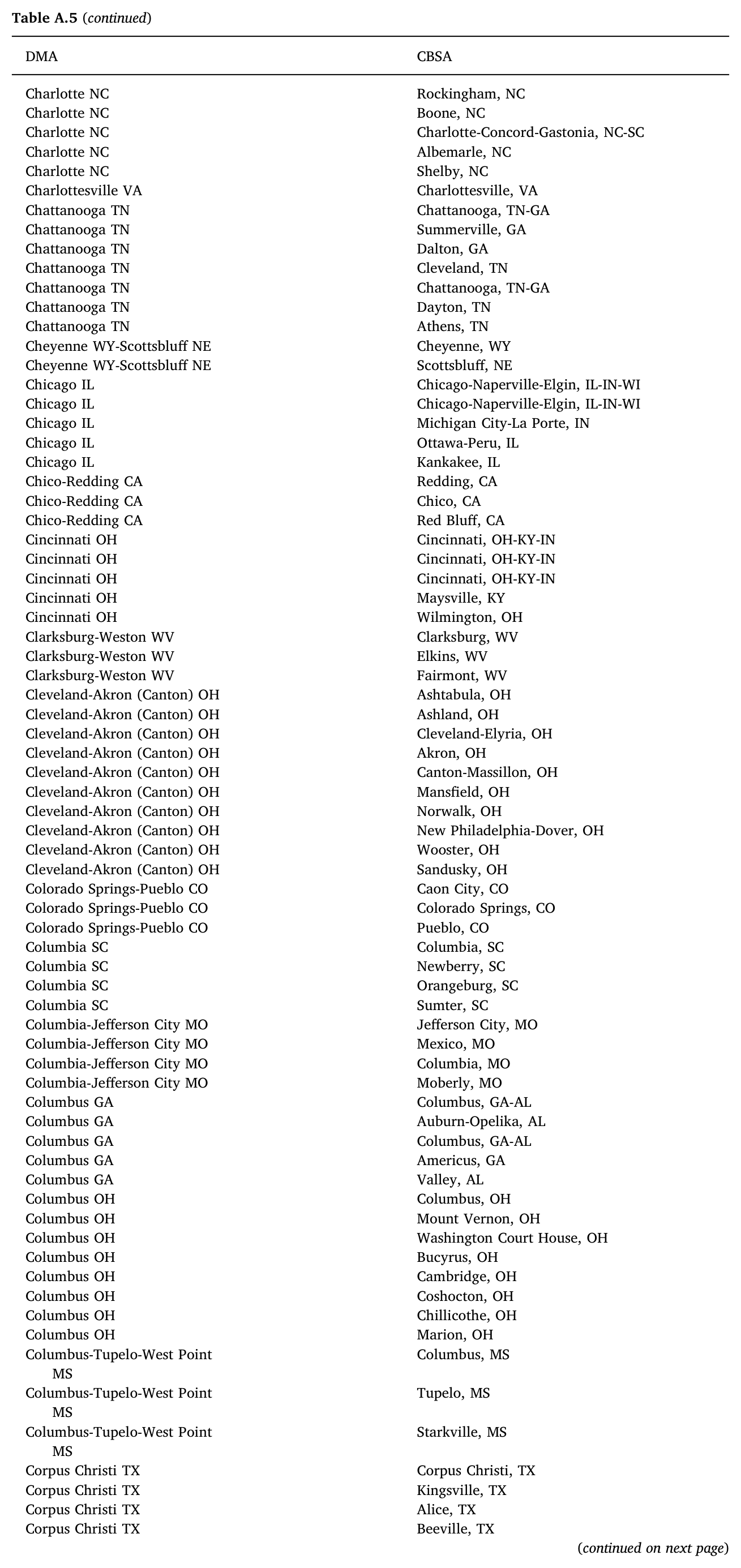
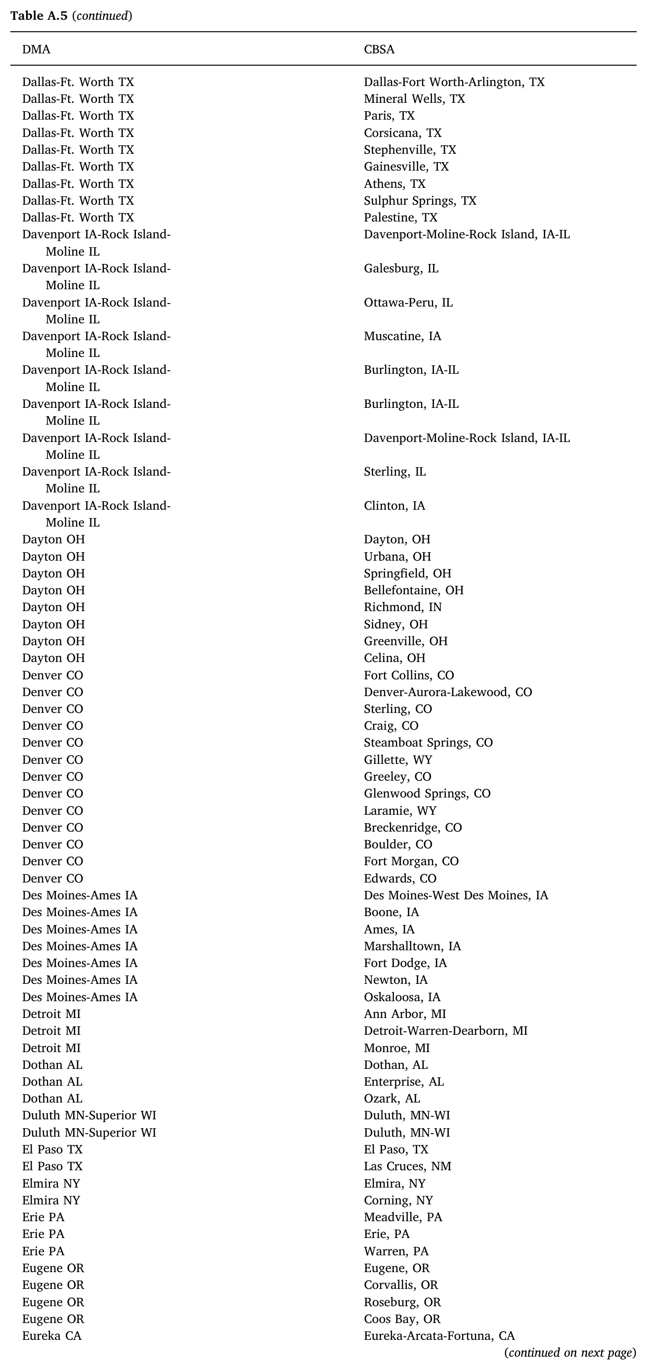
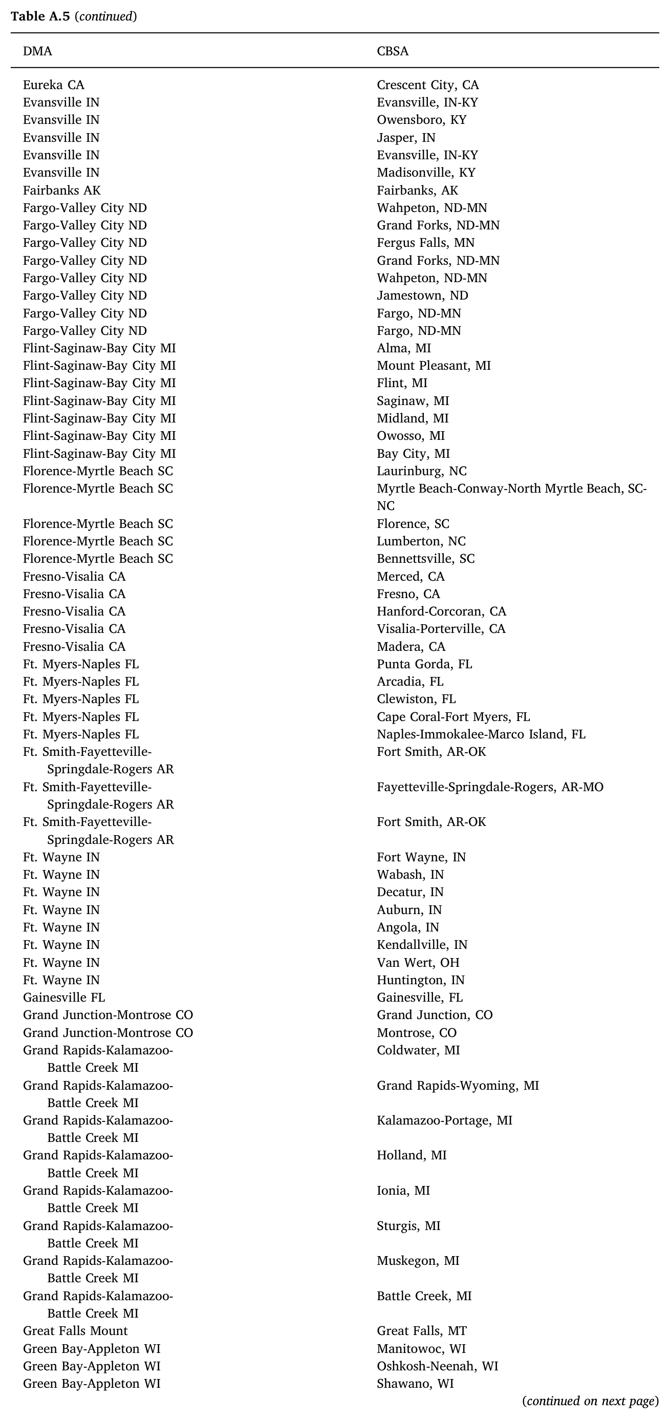
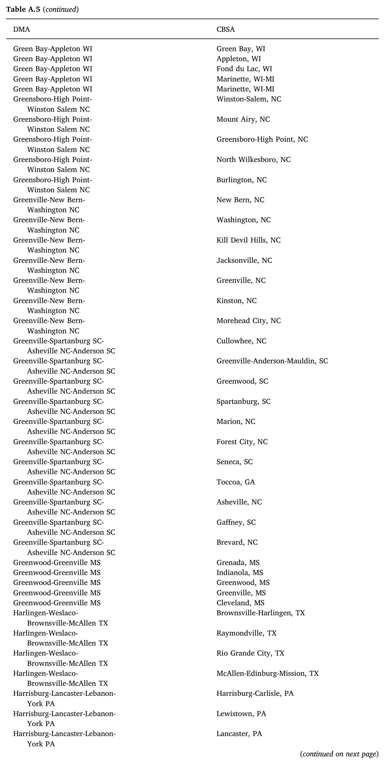
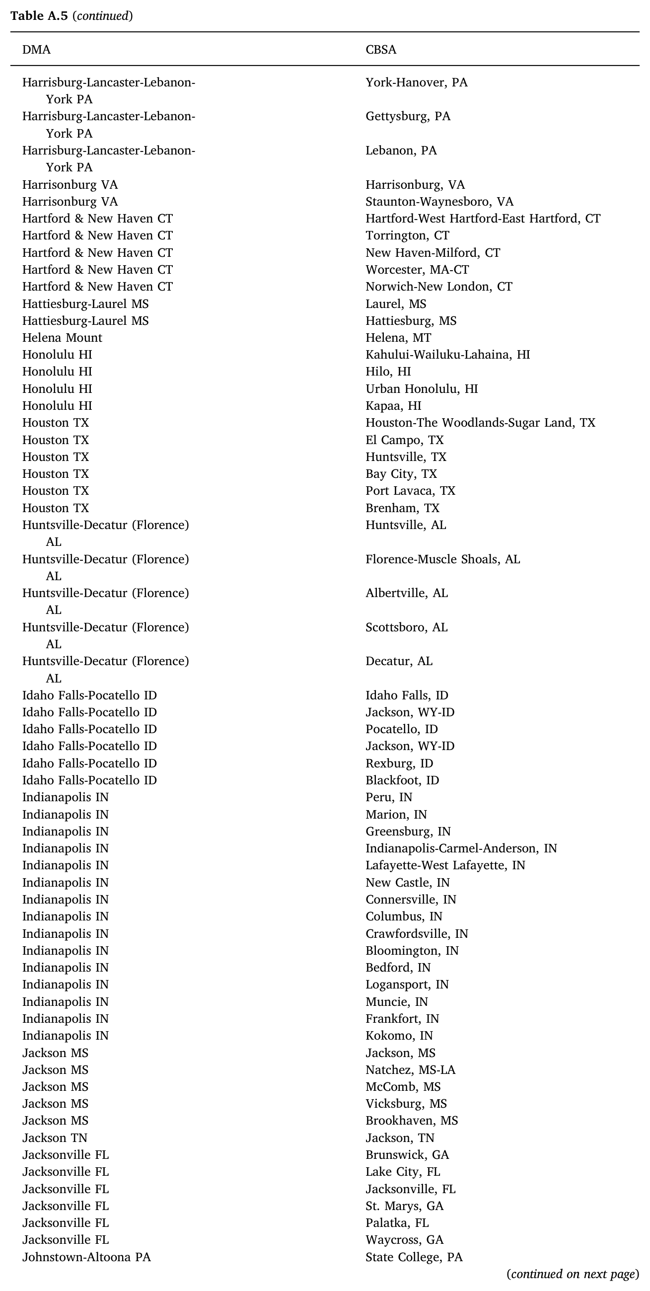
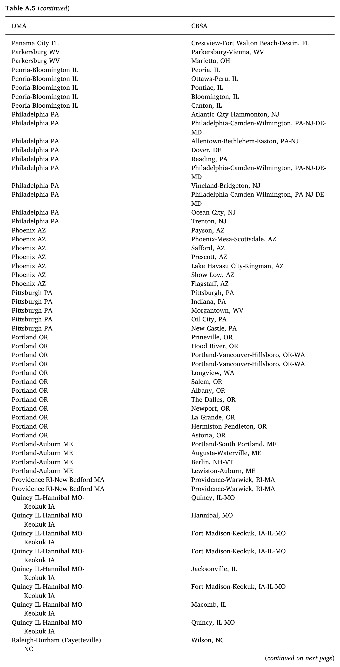
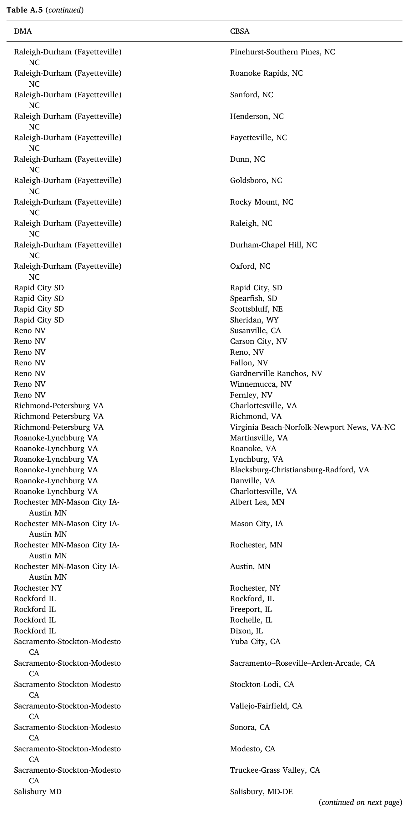
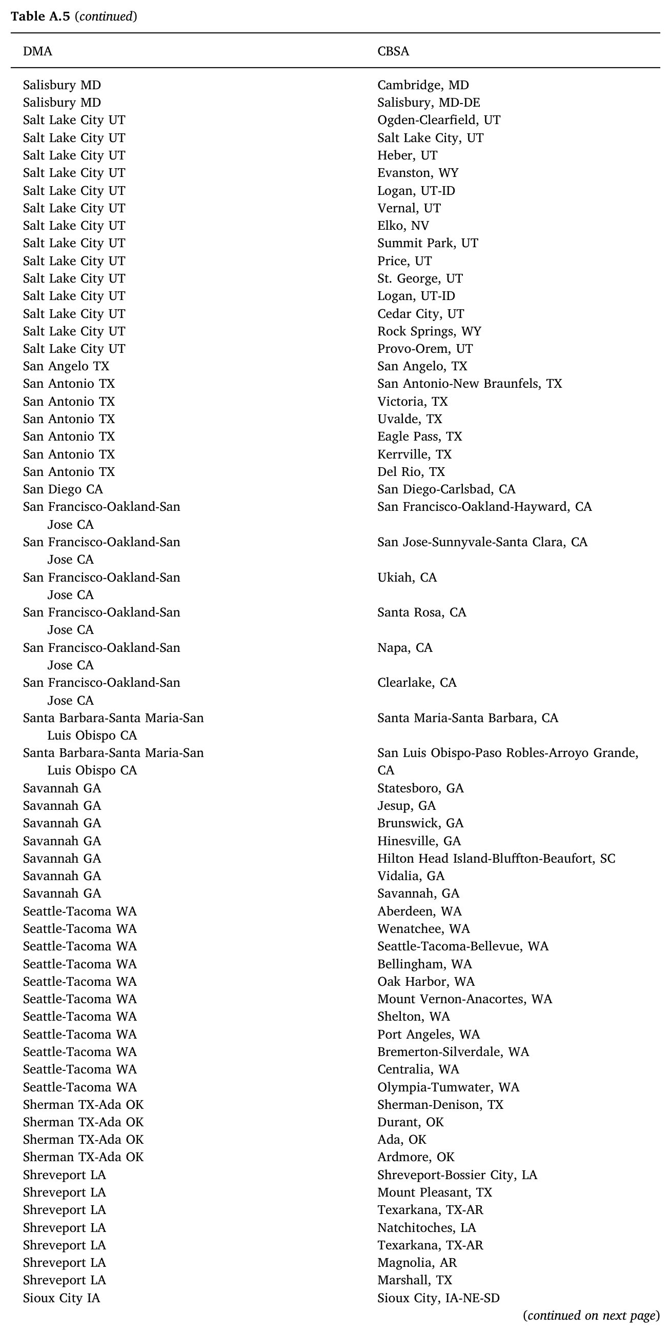
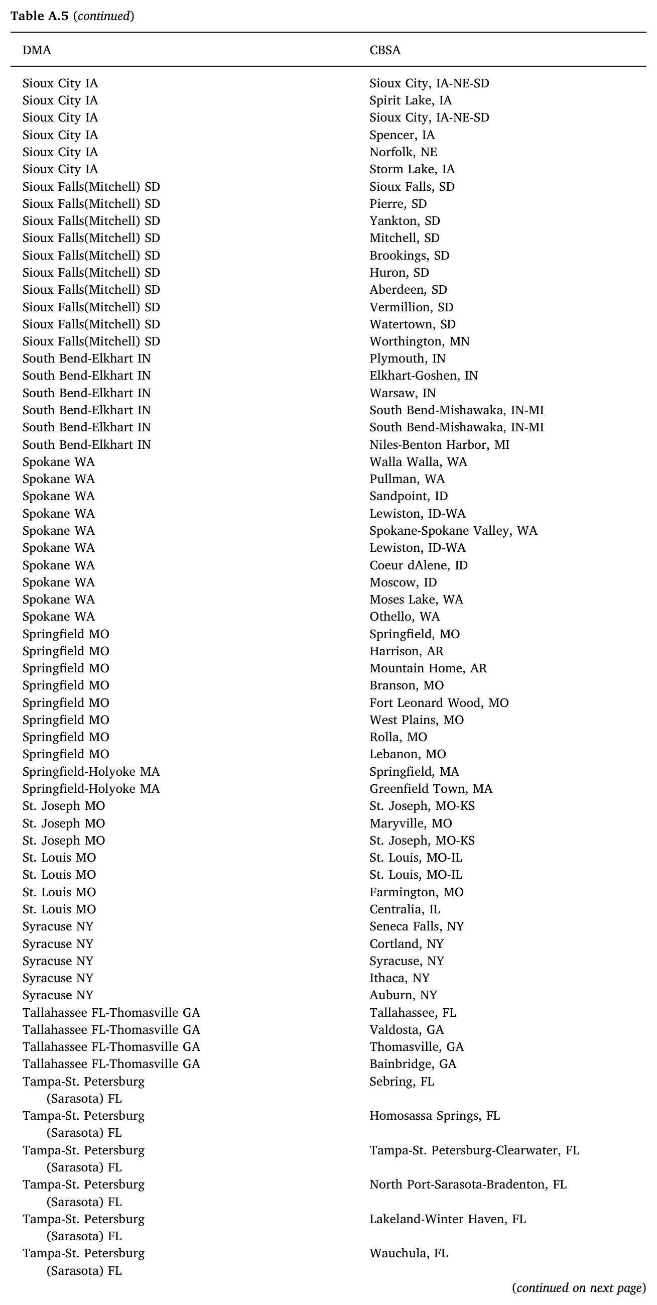
### Table A5. DMA to CBSA crosswalk

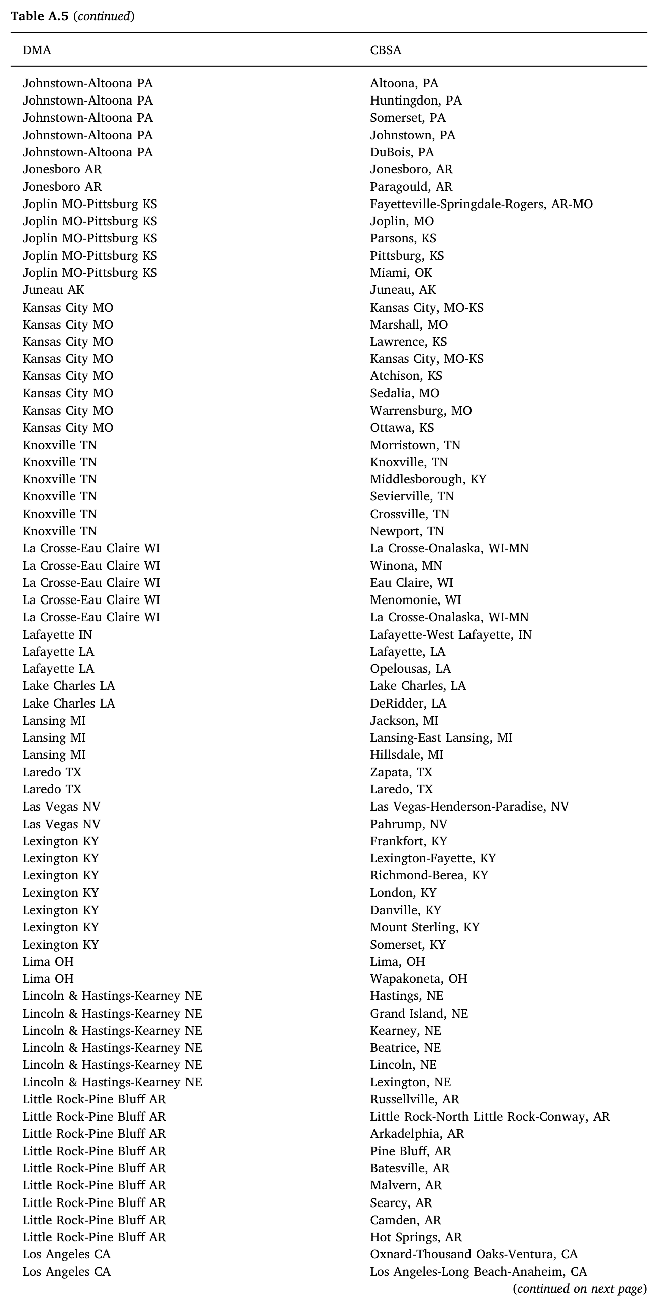
<figure class="article-figure" id="table-a5-page-13"><a href="/files/publications/ay-ja-nfkd4lequxehfrty-assets/table-a5-page-13.png"><img alt="Table A5, panel 1 of 18. Crosswalk from designated market areas to core-based statistical areas, covering DMA entries from Abilene–Sweetwater, Texas through Albany, Georgia." height="578" loading="lazy" src="/files/publications/ay-ja-nfkd4lequxehfrty-assets/table-a5-page-13.png" width="1309"/></a><figcaption>Table A5, supplied PDF page 13. <a href="/files/publications/ay-ja-nfkd4lequxehfrty-assets/table-a5-page-13.png">Open full-resolution image</a>.</figcaption></figure>
<figure class="article-figure" id="table-a5-page-14"><a href="/files/publications/ay-ja-nfkd4lequxehfrty-assets/table-a5-page-14.png"><img alt="Table A5, panel 2 of 18. Crosswalk from designated market areas to core-based statistical areas, covering DMA entries from Albany–Schenectady–Troy, New York through Boise, Idaho." height="2771" loading="lazy" src="/files/publications/ay-ja-nfkd4lequxehfrty-assets/table-a5-page-14.png" width="1309"/></a><figcaption>Table A5 (continued), supplied PDF page 14. <a href="/files/publications/ay-ja-nfkd4lequxehfrty-assets/table-a5-page-14.png">Open full-resolution image</a>.</figcaption></figure>
<figure class="article-figure" id="table-a5-page-15"><a href="/files/publications/ay-ja-nfkd4lequxehfrty-assets/table-a5-page-15.png"><img alt="Table A5, panel 3 of 18. Crosswalk from designated market areas to core-based statistical areas, covering DMA entries from Boise, Idaho through Charlotte, North Carolina." height="2771" loading="lazy" src="/files/publications/ay-ja-nfkd4lequxehfrty-assets/table-a5-page-15.png" width="1309"/></a><figcaption>Table A5 (continued), supplied PDF page 15. <a href="/files/publications/ay-ja-nfkd4lequxehfrty-assets/table-a5-page-15.png">Open full-resolution image</a>.</figcaption></figure>
<figure class="article-figure" id="table-a5-page-16"><a href="/files/publications/ay-ja-nfkd4lequxehfrty-assets/table-a5-page-16.png"><img alt="Table A5, panel 4 of 18. Crosswalk from designated market areas to core-based statistical areas, covering DMA entries from Charlotte, North Carolina through Corpus Christi, Texas." height="2771" loading="lazy" src="/files/publications/ay-ja-nfkd4lequxehfrty-assets/table-a5-page-16.png" width="1309"/></a><figcaption>Table A5 (continued), supplied PDF page 16. <a href="/files/publications/ay-ja-nfkd4lequxehfrty-assets/table-a5-page-16.png">Open full-resolution image</a>.</figcaption></figure>
<figure class="article-figure" id="table-a5-page-17"><a href="/files/publications/ay-ja-nfkd4lequxehfrty-assets/table-a5-page-17.png"><img alt="Table A5, panel 5 of 18. Crosswalk from designated market areas to core-based statistical areas, covering DMA entries from Dallas–Fort Worth, Texas through Eureka, California." height="2771" loading="lazy" src="/files/publications/ay-ja-nfkd4lequxehfrty-assets/table-a5-page-17.png" width="1309"/></a><figcaption>Table A5 (continued), supplied PDF page 17. <a href="/files/publications/ay-ja-nfkd4lequxehfrty-assets/table-a5-page-17.png">Open full-resolution image</a>.</figcaption></figure>
<figure class="article-figure" id="table-a5-page-18"><a href="/files/publications/ay-ja-nfkd4lequxehfrty-assets/table-a5-page-18.png"><img alt="Table A5, panel 6 of 18. Crosswalk from designated market areas to core-based statistical areas, covering DMA entries from Eureka, California through Green Bay–Appleton, Wisconsin." height="2771" loading="lazy" src="/files/publications/ay-ja-nfkd4lequxehfrty-assets/table-a5-page-18.png" width="1309"/></a><figcaption>Table A5 (continued), supplied PDF page 18. <a href="/files/publications/ay-ja-nfkd4lequxehfrty-assets/table-a5-page-18.png">Open full-resolution image</a>.</figcaption></figure>
<figure class="article-figure" id="table-a5-page-19"><a href="/files/publications/ay-ja-nfkd4lequxehfrty-assets/table-a5-page-19.png"><img alt="Table A5, panel 7 of 18. Crosswalk from designated market areas to core-based statistical areas, covering DMA entries from Green Bay–Appleton, Wisconsin through Harrisburg–Lancaster–Lebanon–York, Pennsylvania." height="2599" loading="lazy" src="/files/publications/ay-ja-nfkd4lequxehfrty-assets/table-a5-page-19.png" width="1309"/></a><figcaption>Table A5 (continued), supplied PDF page 19. <a href="/files/publications/ay-ja-nfkd4lequxehfrty-assets/table-a5-page-19.png">Open full-resolution image</a>.</figcaption></figure>
<figure class="article-figure" id="table-a5-page-20"><a href="/files/publications/ay-ja-nfkd4lequxehfrty-assets/table-a5-page-20.png"><img alt="Table A5, panel 8 of 18. Crosswalk from designated market areas to core-based statistical areas, covering DMA entries from Harrisburg–Lancaster–Lebanon–York, Pennsylvania through Johnstown–Altoona, Pennsylvania." height="2599" loading="lazy" src="/files/publications/ay-ja-nfkd4lequxehfrty-assets/table-a5-page-20.png" width="1309"/></a><figcaption>Table A5 (continued), supplied PDF page 20. <a href="/files/publications/ay-ja-nfkd4lequxehfrty-assets/table-a5-page-20.png">Open full-resolution image</a>.</figcaption></figure>
<figure class="article-figure" id="table-a5-page-21"><a href="/files/publications/ay-ja-nfkd4lequxehfrty-assets/table-a5-page-21.png"><img alt="Table A5, panel 9 of 18. Crosswalk from designated market areas to core-based statistical areas, covering DMA entries from Johnstown–Altoona, Pennsylvania through Los Angeles, California." height="2599" loading="lazy" src="/files/publications/ay-ja-nfkd4lequxehfrty-assets/table-a5-page-21.png" width="1309"/></a><figcaption>Table A5 (continued), supplied PDF page 21. <a href="/files/publications/ay-ja-nfkd4lequxehfrty-assets/table-a5-page-21.png">Open full-resolution image</a>.</figcaption></figure>
<figure class="article-figure" id="table-a5-page-22"><a href="/files/publications/ay-ja-nfkd4lequxehfrty-assets/table-a5-page-22.png"><img alt="Table A5, panel 10 of 18. Crosswalk from designated market areas to core-based statistical areas, covering DMA entries from Los Angeles, California through Minot–Bismarck–Dickinson, North Dakota." height="2599" loading="lazy" src="/files/publications/ay-ja-nfkd4lequxehfrty-assets/table-a5-page-22.png" width="1309"/></a><figcaption>Table A5 (continued), supplied PDF page 22. <a href="/files/publications/ay-ja-nfkd4lequxehfrty-assets/table-a5-page-22.png">Open full-resolution image</a>.</figcaption></figure>
<figure class="article-figure" id="table-a5-page-23"><a href="/files/publications/ay-ja-nfkd4lequxehfrty-assets/table-a5-page-23.png"><img alt="Table A5, panel 11 of 18. Crosswalk from designated market areas to core-based statistical areas, covering DMA entries from Minot–Bismarck–Dickinson, North Dakota through Odessa–Midland, Texas." height="2599" loading="lazy" src="/files/publications/ay-ja-nfkd4lequxehfrty-assets/table-a5-page-23.png" width="1309"/></a><figcaption>Table A5 (continued), supplied PDF page 23. <a href="/files/publications/ay-ja-nfkd4lequxehfrty-assets/table-a5-page-23.png">Open full-resolution image</a>.</figcaption></figure>
<figure class="article-figure" id="table-a5-page-24"><a href="/files/publications/ay-ja-nfkd4lequxehfrty-assets/table-a5-page-24.png"><img alt="Table A5, panel 12 of 18. Crosswalk from designated market areas to core-based statistical areas, covering DMA entries from Odessa–Midland, Texas through Panama City, Florida." height="2599" loading="lazy" src="/files/publications/ay-ja-nfkd4lequxehfrty-assets/table-a5-page-24.png" width="1309"/></a><figcaption>Table A5 (continued), supplied PDF page 24. <a href="/files/publications/ay-ja-nfkd4lequxehfrty-assets/table-a5-page-24.png">Open full-resolution image</a>.</figcaption></figure>
<figure class="article-figure" id="table-a5-page-25"><a href="/files/publications/ay-ja-nfkd4lequxehfrty-assets/table-a5-page-25.png"><img alt="Table A5, panel 13 of 18. Crosswalk from designated market areas to core-based statistical areas, covering DMA entries from Panama City, Florida through Raleigh–Durham, North Carolina." height="2565" loading="lazy" src="/files/publications/ay-ja-nfkd4lequxehfrty-assets/table-a5-page-25.png" width="1309"/></a><figcaption>Table A5 (continued), supplied PDF page 25. <a href="/files/publications/ay-ja-nfkd4lequxehfrty-assets/table-a5-page-25.png">Open full-resolution image</a>.</figcaption></figure>
<figure class="article-figure" id="table-a5-page-26"><a href="/files/publications/ay-ja-nfkd4lequxehfrty-assets/table-a5-page-26.png"><img alt="Table A5, panel 14 of 18. Crosswalk from designated market areas to core-based statistical areas, covering DMA entries from Raleigh–Durham, North Carolina through Salisbury, Maryland." height="2599" loading="lazy" src="/files/publications/ay-ja-nfkd4lequxehfrty-assets/table-a5-page-26.png" width="1309"/></a><figcaption>Table A5 (continued), supplied PDF page 26. <a href="/files/publications/ay-ja-nfkd4lequxehfrty-assets/table-a5-page-26.png">Open full-resolution image</a>.</figcaption></figure>
<figure class="article-figure" id="table-a5-page-27"><a href="/files/publications/ay-ja-nfkd4lequxehfrty-assets/table-a5-page-27.png"><img alt="Table A5, panel 15 of 18. Crosswalk from designated market areas to core-based statistical areas, covering DMA entries from Salisbury, Maryland through Sioux City, Iowa." height="2599" loading="lazy" src="/files/publications/ay-ja-nfkd4lequxehfrty-assets/table-a5-page-27.png" width="1309"/></a><figcaption>Table A5 (continued), supplied PDF page 27. <a href="/files/publications/ay-ja-nfkd4lequxehfrty-assets/table-a5-page-27.png">Open full-resolution image</a>.</figcaption></figure>
<figure class="article-figure" id="table-a5-page-28"><a href="/files/publications/ay-ja-nfkd4lequxehfrty-assets/table-a5-page-28.png"><img alt="Table A5, panel 16 of 18. Crosswalk from designated market areas to core-based statistical areas, covering DMA entries from Sioux City, Iowa through Tampa–St. Petersburg–Sarasota, Florida." height="2599" loading="lazy" src="/files/publications/ay-ja-nfkd4lequxehfrty-assets/table-a5-page-28.png" width="1309"/></a><figcaption>Table A5 (continued), supplied PDF page 28. <a href="/files/publications/ay-ja-nfkd4lequxehfrty-assets/table-a5-page-28.png">Open full-resolution image</a>.</figcaption></figure>
<figure class="article-figure" id="table-a5-page-29"><a href="/files/publications/ay-ja-nfkd4lequxehfrty-assets/table-a5-page-29.png"><img alt="Table A5, panel 17 of 18. Crosswalk from designated market areas to core-based statistical areas, covering DMA entries from Terre Haute, Indiana through Washington, DC–Hagerstown, Maryland." height="2565" loading="lazy" src="/files/publications/ay-ja-nfkd4lequxehfrty-assets/table-a5-page-29.png" width="1309"/></a><figcaption>Table A5 (continued), supplied PDF page 29. <a href="/files/publications/ay-ja-nfkd4lequxehfrty-assets/table-a5-page-29.png">Open full-resolution image</a>.</figcaption></figure>
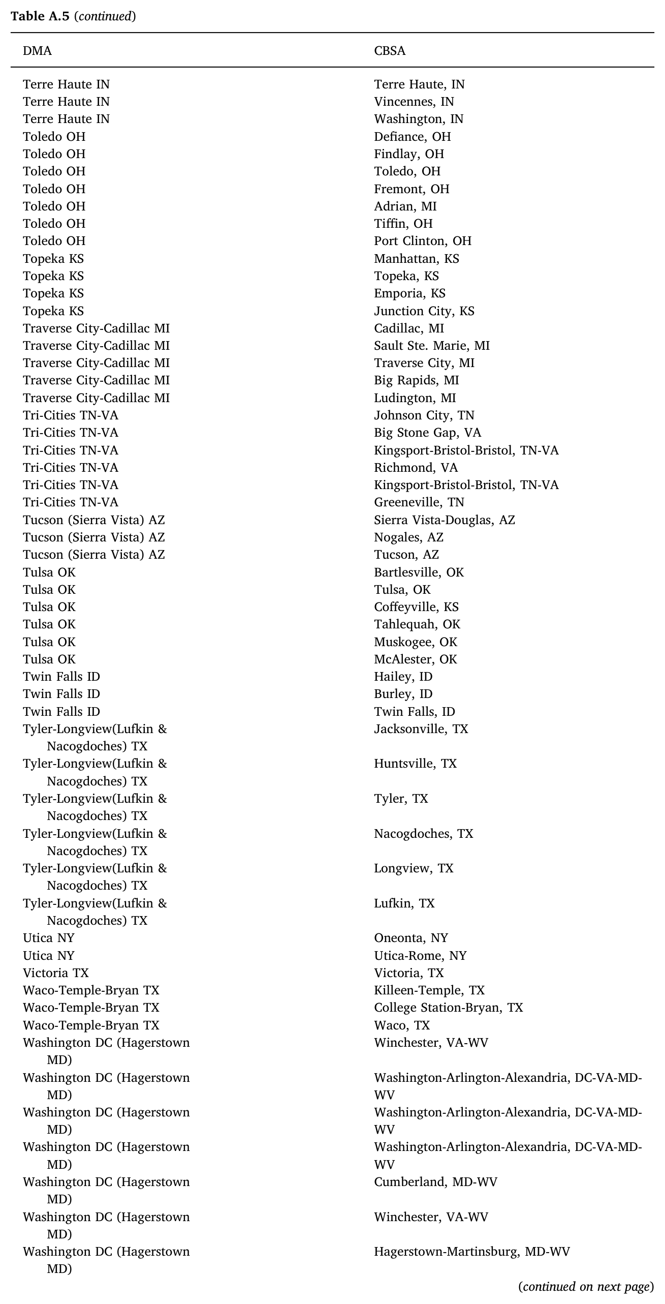
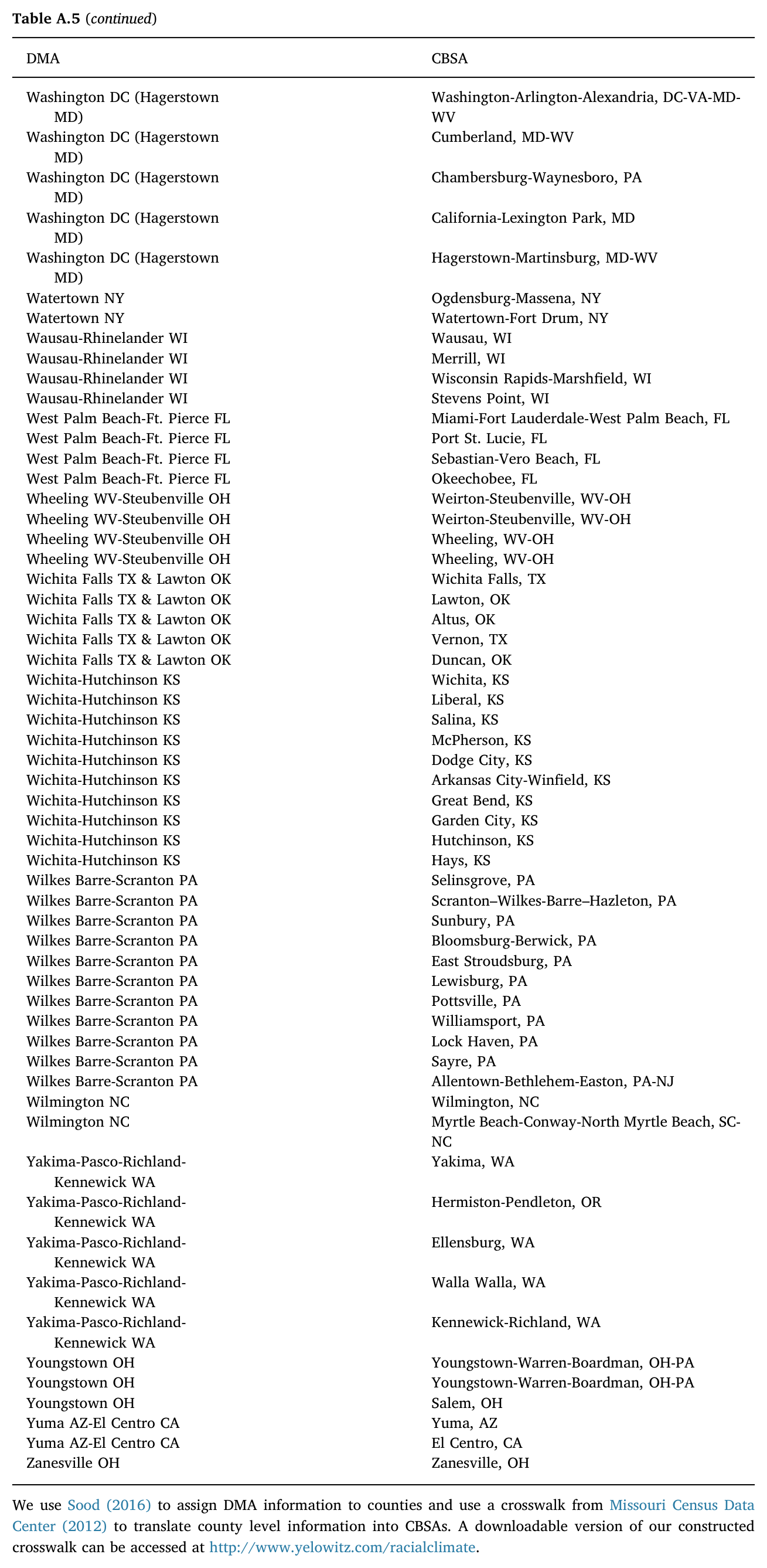
<figure class="article-figure" id="table-a5-page-30"><a href="/files/publications/ay-ja-nfkd4lequxehfrty-assets/table-a5-page-30.png"><img alt="Table A5, panel 18 of 18. Crosswalk from designated market areas to core-based statistical areas, covering DMA entries from Washington, DC–Hagerstown, Maryland through Zanesville, Ohio. Includes the source note describing county-based matching and the historical download address." height="2675" loading="lazy" src="/files/publications/ay-ja-nfkd4lequxehfrty-assets/table-a5-page-30.png" width="1309"/></a><figcaption>Table A5 (continued), supplied PDF page 30. <a href="/files/publications/ay-ja-nfkd4lequxehfrty-assets/table-a5-page-30.png">Open full-resolution image</a>.</figcaption></figure>


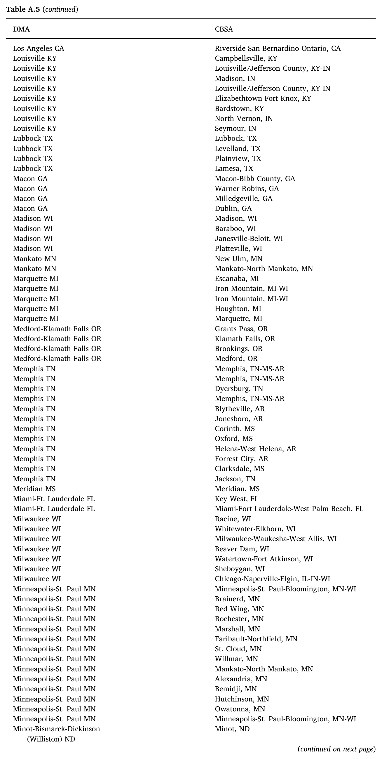
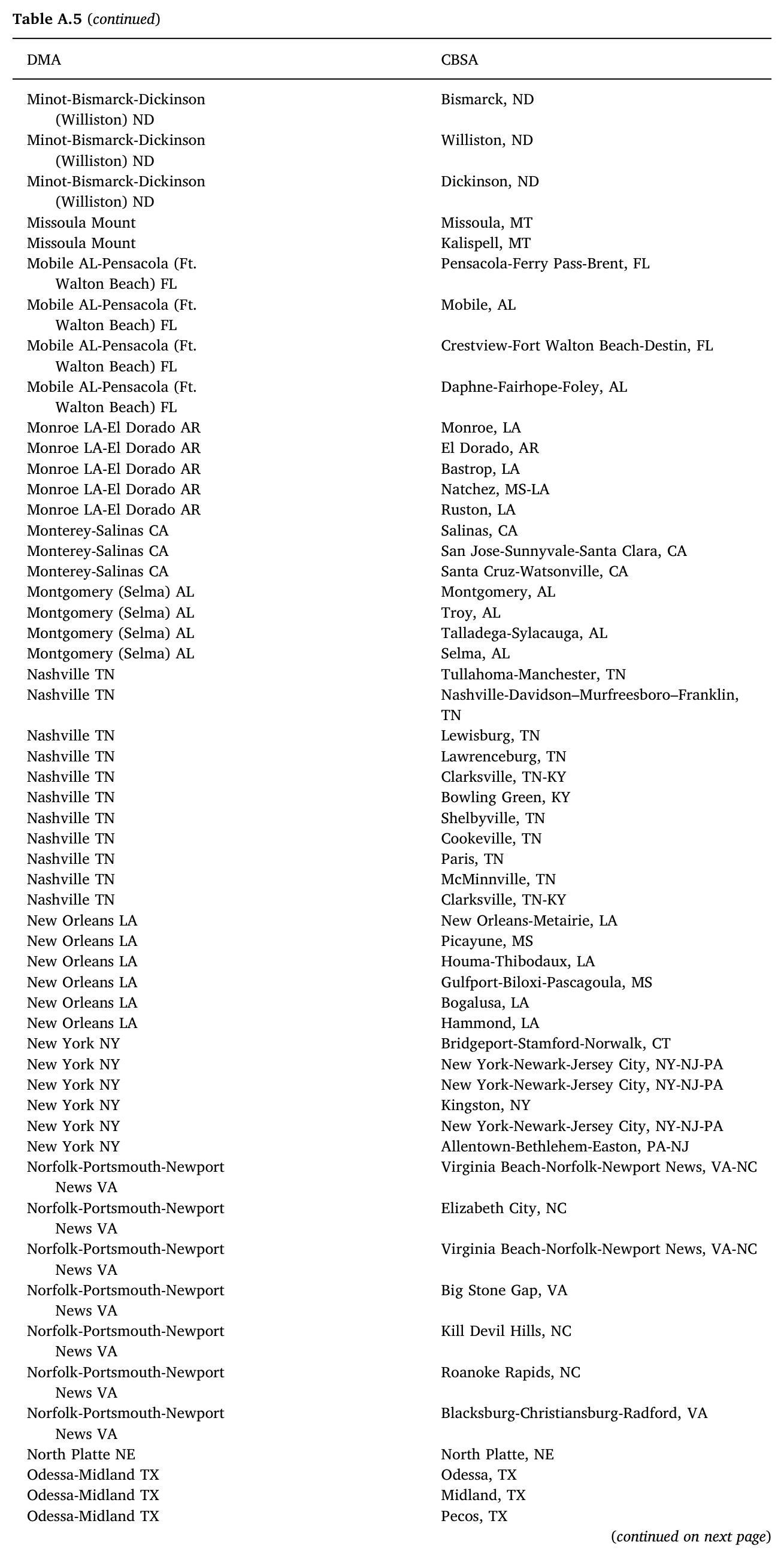
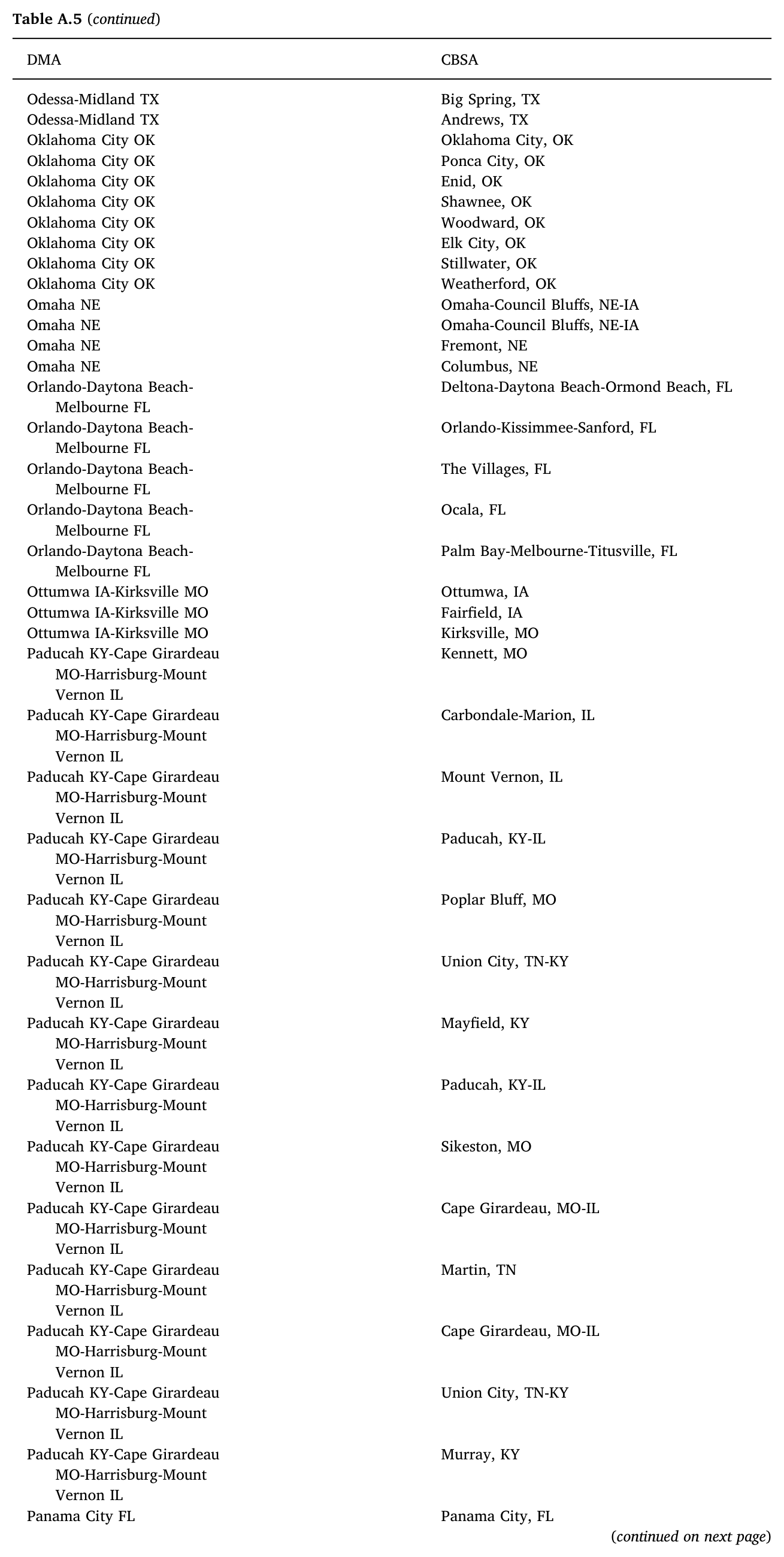
We use Sood (2016) to assign DMA information to counties and use a crosswalk from Missouri Census Data Center (2012) to translate county level information into CBSAs. A downloadable version of our constructed crosswalk can be accessed at http://www.yelowitz.com/racialclimate.


### Figure A1

<figure class="article-figure" id="figure-a1"><a href="/files/publications/ay-ja-nfkd4lequxehfrty-assets/figure-a1.png"><img alt="Figure A1. Six national Google Trends search-intensity series from 2005 through 2017: Black Lives Matter, Michael Brown, Ferguson unrest, Freddie Gray, Trayvon Martin and Tamir Rice. Each series is scaled from zero to 100." height="2340" loading="lazy" src="/files/publications/ay-ja-nfkd4lequxehfrty-assets/figure-a1.png" width="2124"/></a><figcaption>Figure A1, supplied PDF page 31. <a href="/files/publications/ay-ja-nfkd4lequxehfrty-assets/figure-a1.png">Open full-resolution image</a>.</figcaption></figure>


### Figure A2

<figure class="article-figure" id="figure-a2"><a href="/files/publications/ay-ja-nfkd4lequxehfrty-assets/figure-a2.png"><img alt="Figure A2. Map of 2012 metropolitan crime intensity, shaded in five Z-score groups from −2.15 to 2.4, using FBI Uniform Crime Report statistics." height="864" loading="lazy" src="/files/publications/ay-ja-nfkd4lequxehfrty-assets/figure-a2.png" width="2124"/></a><figcaption>Figure A2, supplied PDF page 32. <a href="/files/publications/ay-ja-nfkd4lequxehfrty-assets/figure-a2.png">Open full-resolution image</a>.</figcaption></figure>

## References

Antonovics, K.L., Sander, R.H., 2013. Affirmative action bans and the chilling effect. Am. Law Econ. Rev. 15 (1), 252–299.

Bayer, P., Ferreira, F., Ross, S.L., 2016. The vulnerability of minority homeowners in the housing boom and bust. Am. Econ. J.: Econ. Policy 8 (1), 1–27. http://dx.doi.org/10.1257/pol.20140074.

Bostic, R.W., Lee, K.O., 2008. Mortgages, risk, and homeownership among low- and moderate-Income families. Am. Econ. Rev. 98 (2), 310–314.

Chaney, C., Robertson, R.V., 2013. Racism and police brutality in america. J. Afr. Am. Stud. 17 (4), 480–505.

Chetty, R., Friedman, J.N., Hilger, N., Saez, E., Schanzenbach, D.W., Yagan, D., 2011. How does your kindergarten classroom affect your earnings? evidence from project star. Q. J. Econ. 126 (4), 1593. http://dx.doi.org/10.1093/qje/qjr041.

Courtemanche, C., Marton, J., Ukert, B., Yelowitz, A., Zapata, D., 2017. Early impacts of the affordable care act on health insurance coverage in medicaid expansion and non-Expansion states. J. Policy Anal. Manag. 36 (1), 178–210. http://dx.doi.org/10.1002/pam.21961.

Cutler, D.M., Glaeser, E.L., 1997. Are ghettos good or bad? Q. J. Econ. 112 (3), 827. http://dx.doi.org/10.1162/003355397555361.

Davis, M.A., 2012. Questioning homeownership as a public policy goal. Cato Policy Anal. Accessed from: https://object.cato.org/sites/cato.org/files/pubs/pdf/PA696.pdf

Deng, Y., Ross, S.L., Wachter, S.M., 2003. Racial differences in homeownership: the effect of residential location. Reg. Sci. Urban Econ. 33 (5), 517–556.

DiPasquale, D., Glaeser, E.L., 1999. Incentives and social capital: are homeowners better citizens? J. Urban Econ. 45 (2), 354–384.

Ekins, E. E., 2016. Policing in america: understanding public attitudes toward the police. results from a national survey. Working Paper.

Fryer, R.G., 2016. An Empirical Analysis of Racial Differences in Police Use of Force. Technical Report. National Bureau of Economic Research.

Gelbach, J.B., 2016. When do covariates matter? and which ones, and how much? J. Labor Econ. 34 (2), 509–543. http://dx.doi.org/10.1086/683668.

Haurin, D.R., Parcel, T.L., Haurin, R.J., 2002. Does homeownership affect child outcomes? Real Estate Econ. 30 (4), 635–666.

Holupka, S., Newman, S.J., 2012. The effects of homeownership on Children’s outcomes: real effects or self-Selection? Real Estate Econ. 40 (3), 566–602. http://dx.doi.org/10.1111/j.1540-6229.2012.00330.x.

Ihlanfeldt, K.R., 1981. An empirical investigation of alternative approaches to estimating the equilibrium demand for housing. J. Urban Econ. 9 (1), 97–105.

Kling, J.R., Liebman, J.B., Katz, L.F., 2007. Experimental analysis of neighborhood effects. Econometrica 75 (1), 83–119.

Missouri Census Data Center, 2012. MABLE/Geocorr[90-2k-12-14], Version 1.2 Geographic Correspondence Engine. http://mcdc.missouri.edu/websas/geocorr12.html.

Munnell, A.H., Tootell, G.M., Browne, L.E., McEneaney, J., 1996. Mortgage lending in boston: interpreting HMDA data. Am. Econ. Rev. 86 (1), 25–53.

Ondrich, J., Ross, S., Yinger, J., 2001. Geography of housing discrimination. J. Hous. Res. 12 (2), 217–238.

Ondrich, J., Ross, S., Yinger, J., 2003. Now you see it, now you don’t: why do real estate agents withhold available houses from black customers? Rev. Econ. Stat. 85 (4), 854–873.

Poterba, J., Sinai, T., 2008. Tax expenditures for owner-occupied housing: deductions for property taxes and mortgage interest and the exclusion of imputed rental income. Am. Econ. Rev. 98 (2), 84–89.

Ross, S.L., Tootell, G.M., 2004. Redlining, the community reinvestment act, and private mortgage insurance. J. Urban Econ. 55 (2), 278–297. http://dx.doi.org/10.1016/S0094-1190(02)00508-9.

Ruggles, S., Genadek, K., Goeken, R., Grover, J., Sobek, M., 2015. Integrated public use microdata series: version 6.0 2000 migration pumas and super-pumas. Minneapolis: University of Minnesota. http://doi.org/10.18128/D010.V6.0.

Shapiro, T.M., 2006. Race, homeownership and wealth. Wash. Univ. J. Law Policy 20, 53–74.

Sidhu, D.S., 2007. The chilling effect of government surveillance programs on the use of the internet by muslim-Americans. Univ. Maryland Law J. Race, Relig., Gender Class 7 (2), 375–393. Accessed from: http://digitalcommons.law.umaryland.edu/rrgc/vol7/iss2/10.

Sinai, T., Souleles, N.S., 2005. Owner-occupied housing as a hedge against rent risk. Q. J. Econ. 120 (2), 763–789.

Sood, G., 2016. Geographic Information on Designated Media Markets. https://doi.org/10.7910/DVN/IVXEHT.

Stephens-Davidowitz, S., 2013. Unreported victims of an economic downturn. Working Paper.

Stephens-Davidowitz, S., 2014. The cost of racial animus on a black candidate: evidence using google search data. J. Public Econ. 118, 26–40.

Stephens-Davidowitz, S., 2017. Everybody Lies: Big Data, New Data, and What the Internet can Tell us About who we Really Are. HarperCollins.

Tootell, G., 1996. Redlining in boston: do mortgage lenders discriminate against neighborhoods? Q. J. Econ. 111 (4), 1049–1079.

Turner, M.A., Santos, R., Levy, D.K., Wissoker, D., Aranda, C., Pitingolo, R., 2013. Housing discrimination against racial and ethnic minorities 2012. Washington, DC: Urban Institute, Department of Housing and Urban Development. Accessed from: https://www.huduser.gov/portal/Publications/pdf/HUD--514_HDS2012.pdf.

Turner, T.M., Luea, H., 2009. Homeownership, wealth accumulation and income status. J. Hous. Econ. 18 (2), 104–114. http://dx.doi.org/10.1016/j.jhe.2009.04.005.

Watson, T., 2014. Inside the refrigerator: immigration enforcement and chilling effects in medicaid participation. Am. Econ. J.: Econ. Policy 6 (3), 313–338.

Yelowitz, A., 2007. Young adults leaving the nest: the role of cost-of-living. The Price of Independence: The Economics of Early Adulthood. Russell Sage, pp. 170–206.

Yelowitz, A., 2017. Local housing costs and basic household needs. Empir. Econ. 52 (3), 901–923. http://dx.doi.org/10.1007/s00181-016-1185-2.

Yelowitz, A., Wilson, M., 2015. Characteristics of bitcoin users: an analysis of google search data. Appl. Econ. Lett. 22 (13), 1030–1036.

## Notes

<p id="source-note-1"><strong>1.</strong> We thank Stephen Ross and anonymous referees for helpful comments.</p>

<p id="source-note-2"><strong>2.</strong> Sinai and Souleles (2005) find that the probability of homeownership increases faster with rent volatility for long-horizon households than for short-horizon households.</p>

<p id="source-note-3"><strong>3.</strong> However, Holupka and Newman (2012) argue that such beneficial homeownership effects may be due to selection bias.</p>

<p id="source-note-4"><strong>4.</strong> See http://www.presidency.ucsb.edu/ws/?pid=25063.</p>

<p id="source-note-5"><strong>5.</strong> See https://www.census.gov/housing/hvs/files/annual16/ann16t_22.xlsx.</p>

<p id="source-note-6"><strong>6.</strong> See https://www.nytimes.com/2016/08/21/us/milwaukee-segregation-wealthy-black-families.html for an example of black households locating in less racially charged areas leading to segregation. Presumably, racial climate also influences the decision to locate/invest in homeownership across cities and not just within cities.</p>

<p id="source-note-7"><strong>7.</strong> Other examples include internet use by Muslim-Americans in the aftermath of the September 11th attacks (Sidhu, 2007) and college applications following affirmative action bans (Antonovics and Sander, 2013).</p>

<p id="source-note-8"><strong>8.</strong> Watson (2014) proxies for the chilling effect on Medicaid participation for children of immigrants using spatial and temporal variation in federal enforcement actions from the Immigration and Naturalization Service.</p>

<p id="source-note-9"><strong>9.</strong> See http://blacklivesmatter.com/herstory/</p>

<p id="source-note-10"><strong>10.</strong> There are a total of 210 DMA in the U.S., which correspond to different media markets as defined by Nielsen. We use Sood (2016) to assign DMA information to counties and use a crosswalk from Missouri Census Data Center (2012) to translate county level information into metro areas. Appendix Table A.5 lists the final crosswalk between DMA and CBSA. In addition, a downloadable version of our constructed crosswalk can be accessed at http://www.yelowitz.com/racialclimate. For our sample, an average of roughly two metro areas map into a single DMA. In the analysis, we cluster at the DMA level.</p>

<p id="source-note-11"><strong>11.</strong> We use the average indexes for these measures over time rather than exploiting any time variation in the metrics. The average Z-score is created by subtracting the mean and dividing by the standard deviation for each of the search terms. We then sum the scores and divide by the standard deviation of the sum to get an index of mean zero and standard deviation one (Chetty et al., 2011; Kling et al., 2007).</p>

<p id="source-note-12"><strong>12.</strong> See Appendix Fig. A.1 for an illustration of the timing of search interest in each event/topic.</p>

<p id="source-note-13"><strong>13.</strong> We use data on 2-Bedroom Units at the county level. For counties with sub-areas reported, we weight the areas by their population in 2010 to aggregate to the county level. These are then mapped into metro areas. Data accessed from https://www.huduser.gov/portal/datasets/fmr.html.</p>

<p id="source-note-14"><strong>14.</strong> For the HPI we use Metropolitan Statistical Areas and Divisions (Not Seasonally Adjusted) estimated using Sales Prices and Appraisal data. We average across quarters to get an annual measure and normalize the measure to be 100 in 2005. Data accessed from https://www.fhfa.gov/DataTools/Downloads/Pages/House-Price-Index-Datasets.aspx#mpo.</p>

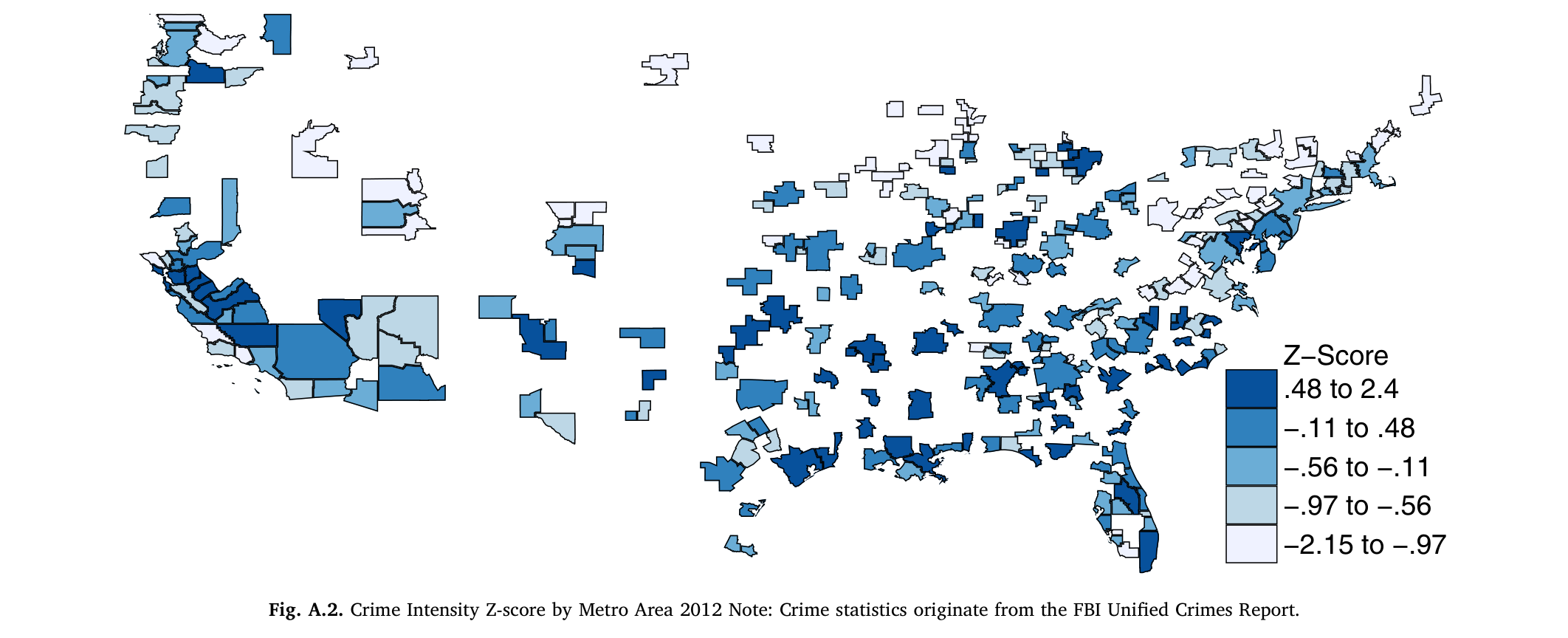
<p id="source-note-15"><strong>15.</strong> From the crime data, we create a crime Z-score calculated in a similar fashion as the racial climate index using statistics on violent crimes, murder/non-negligent manslaughter, robbery, aggravated assault, property crime burglary and motor vehicle thefts by metro area. See Fig. A.2 for a map of the crime Z-score.</p>

<p id="source-note-16"><strong>16.</strong> We exclude all micropolitan areas and areas and Public Use Micro Areas that do not map into a core-based statistical area (CBSA).</p>

<p id="source-note-17"><strong>17.</strong> Economic theory predicts that households should only respond to changing racial climate in the short-run inasmuch the costs of a poor racial climate exceeds moving costs (Ihlanfeldt, 1981).</p>

<p id="source-note-18"><strong>18.</strong> For example, low rates of black homeownership could result in more searches related to the racially charged events.</p>

<p id="source-note-19"><strong>19.</strong> Nearly identical results were obtained for the main specification using a Probit model rather than a linear probability model.</p>

<p id="source-note-20"><strong>20.</strong> Yelowitz (2007) and Yelowitz (2017) examine the impacts of house prices and rents at the local level over time using data from FHFA and HUD.</p>

<p id="source-note-21"><strong>21.</strong> The discussion of this second factor relies on the assumption that potential homeowners exhibit this behavior more than renters. Given the investment associated with homeownership, this is likely a reasonable assumption.</p>

<p id="source-note-22"><strong>22.</strong> The main results are robust to conducting the analysis using the top and bottom terciles and quintiles. The coefficient on racial climate is larger in absolute magnitude (more negative) using the top and bottom quintiles and slightly smaller using the top and bottom terciles. The results are presented in Appendix Table A.2.</p>

<p id="source-note-23"><strong>23.</strong> These results are sensitive to the inclusion of metro controls by race interactions. In Appendix Table A.3 we present the results from a Gelbach Decomposition of the influence of each covariate on the racial climate index (Gelbach, 2016). The findings show that interaction of race with Percent Black is the primary covariate that cause the point estimate on the racial climate variable to change from a small insignificant negative to a statistically significant and more negative result when the interactions are added.</p>

<p id="source-note-24"><strong>24.</strong> The results are reported in Appendix Table A.4.</p>

<p id="source-note-25"><strong>25.</strong> Household observations are mapped into MIGPUMAS using Ruggles et al. (2015). We exclude observations where there are not at least 100 observations for the particular location/demographic cell. Overall, households are mapped into 26,497 unique cells based on demographics, and former locations. Homeownership rates are calculated using the ACS from 2005 to 2015.</p>

<p id="source-note-26"><strong>26.</strong> In addition, we include the first measure of the likelihood of previous homeownership (based on age and income) in each specification.</p>

<p id="source-note-27"><strong>27.</strong> The results from the specification without the control for the interaction of race and the previous racial climate restricted to the same sample yields a statistically significant point estimate of −8.2 percentage points.</p>

<p id="source-note-28"><strong>28.</strong> We use Summary File 1 (SF1) Urban-Rural Update files accessed through http://www.ciser.cornell.edu/pub/2010SF1/census2010sf1.shtm.</p>