# Life Insurance Holdings and Well-Being of Surviving Spouses

**Authors:** Timothy F. Harris and Aaron Yelowitz  
**Citation:** Timothy F. Harris and Aaron Yelowitz (2018). Life Insurance Holdings and Well-Being of Surviving Spouses. Contemporary Economic Policy 36(3): 526–538. DOI: 10.1111/coep.12211.

© 2016 Western Economic Association International. Online Early publication November 18, 2016.  

**Author information:** Timothy F. Harris — Ph.D. Candidate, Department of Economics, University of Kentucky, Gatton College of Business and Economics, Lexington, KY; phone (801) 710-9910; email tim.harris@uky.edu. Aaron Yelowitz — Associate Professor, Department of Economics, University of Kentucky, Gatton College of Business and Economics, Lexington, KY; phone (859) 257-7634; fax (859) 323-1920; email aaron@uky.edu.

## Abstract

Premature death of a breadwinner can have devastating financial consequences on surviving dependents. This study investigates the role of life insurance in mitigating the long-run financial consequences of spousal mortality. Using the Health and Retirement Study, we examine individuals whose spouses died during or soon after his or her peak earnings years. After controlling for socioeconomic status, we find that sizable lump-sum life insurance payouts do not significantly influence spousal well-being.
**JEL classification:** D31; G22; I31; J32; J33; J38


### ABBREVIATIONS

- **DC:** Defined Contribution
- **ESLI:** Employer-Sponsored Life Insurance
- **FPL:** Federal Poverty Line
- **HRS:** Health and Retirement Study
- **NDI:** National Death Index
- **SNAP:** Supplemental Nutrition Assistance Program
- **SSI:** Supplemental Security Income

## I. INTRODUCTION
Death of a breadwinner can have catastrophic financial consequences for surviving dependents. In the United States, there are high rates of widow poverty with one in five widows being below the federal poverty line (FPL) and evidence of increased labor force participation by surviving dependents (Sevak, Weir, and Willis 2004; Elliott and Simmons 2011; Fadlon and Nielsen 2015). Consequences from premature death like higher poverty, increased labor supply, increased remarriage rates, or reliance on relatives can be mitigated by holding life insurance. To what extent does life insurance fulfill the classic “consumption smoothing” role, in turn reducing other distortions? Although several studies have speculated that increased life insurance coverage would reduce the incidence of poverty for surviving spouses (Auerbach and Kotlikoff 1991; Bernheim et
al. 2003), there has been, to date, no direct evidence.

Our study provides such evidence on how life insurance payouts influence surviving spouses, by using 20 years of data from the Health and Retirement Study (HRS). The HRS contains detailed financial information including payouts from life insurance policies and accurate information on the precise date of death. We analyze the well-being of individuals whose
spouses died during or soon after his or her peak earnings years, and examine the elderly individual’s financial status 3 years following the spouse’s death. We find significant effects of lump-sum life insurance payouts on the well-being of surviving spouses without controlling for socioeconomic factors. Once we control for such factors, there is no significant reduction of poverty for surviving spouses except in the case of very small payouts that are likely provided through employer-sponsored life insurance (ESLI). These findings are consistent with the idea that life insurance payouts are simply a proxy for financial savviness, but do not cause higher long-run financial well-being. One possible explanation for this result is that surviving spouses spend the large financial windfall from life
insurance very quickly, mitigating its effect in the medium or long run. Our findings suggest that large lump-sum life insurance payouts may be less effective than annuitized payouts.

In addition to the policy importance, our findings contribute to a literature where commonly assumed causal relationships are either diminished or eliminated with the inclusion of additional covariates, balanced samples, or instrumental variable techniques. Examples include the consequences of subsidized housing (Currie and Yelowitz 2000), military service (Angrist 1990), arrests (Grogger 1995), substance use (Rees, Argys, and Averett 2001), teen pregnancy (Hotz, McElroy, and Sanders 2005), and depression (Cseh 2008).

The remainder of the paper is organized as follows. Section II provides an overview of life insurance markets. Section III describes the data. Section IV provides the empirical specification. Section V presents and discusses our results. Section VI concludes.
## II. LIFE INSURANCE MARKETS
Institutional features of the life insurance markets are important for understanding life insurance’s influence on the well-being of surviving spouses. Individuals generally pay an annual premium, and their heirs receive a payment if the insured individual dies while covered by life insurance. In 2014, life insurance coverage totaled $20.1 trillion originating from individual and group market coverage (American Council of Life Insurers 2015).

Consumers purchase individual market coverage directly through the insurer and individual coverage constituted 59% of all life insurance in 2014. Individual life insurance is mainly separated into term and whole life coverage policies. Term life insurance provides coverage for a specified period of time (typically ranging from 10 to 30 years) and pays the face value of the policy upon death of the policyholder. Term life insurance accounts for 70% of the face value of individual life insurance policies, while only accounting for 39% of individual policies (American Council of Life Insurers 2015). Whole life insurance provides coverage for life and has an investment portion that accumulates a cash value over time.

Group coverage is the other major source of life insurance and constitutes 41% of all life insurance coverage (American Council of Life Insurers 2015). Group coverage generally originates through an employer and is known as ESLI. For employed adults, 53% have some ESLI coverage and 24% exclusively have ESLI coverage.<sup><a href="#source-note-1" aria-label="Source note 1">1</a></sup> In comparison to individual market coverage, the average face value for ESLI coverage purchased
in 2014 was over $100,000 less than the average individual life insurance policy (American Council of Life Insurers 2015). The standard form of payment for group life insurance is a lump-sum distribution (Grossman 1992). ESLI typically has an automatic portion provided by the employer (basic coverage) and an option to purchase additional coverage through payroll deductions (supplemental coverage). Basic coverage is generally provided as a multiple of salary or a flat dollar amount and does not require employee contribution for 95% of covered workers (U.S. Department of Labor 2015). For the non-trivial portion of employers that offer basic coverage as a flat dollar amount, the average level was $16,329 from 1990 to 1997 with 25% being less than $10,000 in 2015.<sup><a href="#source-note-2" aria-label="Source note 2">2</a></sup> In addition, it is typical for basic ESLI to decrease
as an employee ages. For example, 56% of ESLI plans for full-time workers imposed benefit reductions for older workers in 1988 (Bellet 1989).<sup><a href="#source-note-3" aria-label="Source note 3">3</a></sup> Consequently, basic coverage—the automatic portion—can be very small for workers approaching retirement age. In contrast to individual life insurance payouts, basic ESLI payouts can occur without any financial planning on the part of the individual.

Although ESLI and individual market coverage are close substitutes, there appears to be minimal crowd-out between individual and ESLI coverage (Harris and Yelowitz 2016). Consequently, increased ESLI generally translates into increased total life insurance coverage.
## III. DATA
We use longitudinal data from the HRS from 1992 to 2012 to analyze the effect of life insurance on the well-being of surviving spouses. For consistency across survey years, we use the RAND HRS data file (version O) supplemented by the original HRS data files.<sup><a href="#source-note-4" aria-label="Source note 4">4</a></sup> The HRS uses both exit interviews completed by surviving relatives and merged information from the National Death Index (NDI) to ascertain accurate mortality information. There are 37,317 unique individuals surveyed from 1992 to 2012. We restrict the sample to individuals that reported being married during the sample years ( _N_ = 26,037). In addition, we restrict the sample to widows or widowers whose spouses died during or soon after the peak earning years (deaths between age 55 and 68) who we observe 3 years following their spouse’s death without missing values (423 surviving spouses).<sup><a href="#source-note-5" aria-label="Source note 5">5</a></sup>


The HRS sample started in 1992 with individuals aged 51–61. At that time, average life expectancy, conditional on living to age 51, was 77 for men and 82 for women.<sup><a href="#source-note-6" aria-label="Source note 6">6</a></sup> Of the individuals who died between age 55 and 68, nearly 60% reported having better than a 50% chance of living to 75. Therefore, our sample consists of widows and widowers whose spouses had premature deaths, the majority of which were unexpected. To the extent that large life insurance payouts would serve a consumption smoothing role, it would be for such premature, unexpected deaths.

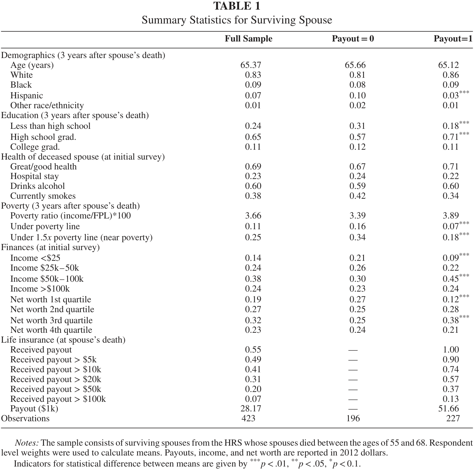
Table 1 shows the summary statistics for individuals as measured 3 years following their spouse’s death. The sample is predominantly white and approximately three-quarters have at least a high school education. A little over half of the sample received life insurance payouts. However, many of these policies were relatively small and only 30% received payouts greater than $20,000.<sup><a href="#source-note-7" aria-label="Source note 7">7</a></sup> Conditional on receiving a life insurance payout, the mean payout was $50,031. Table 1 additionally highlights some of the differences between households and individuals that receive payouts and those that do not receive payouts. Those that receive payouts are less likely to be Hispanic, more likely to graduate from high school, and are significantly less likely to be impoverished. Additionally, those that received payouts are less likely to
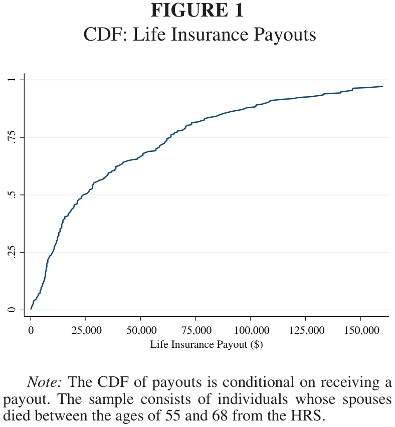
be in the lowest income bin and the lowest quartile for net worth. Figure 1 further shows that distribution of payouts conditional on receiving one.

Approximately half off all individuals that were awarded a payout received less than $25,000.
### Table 1. Summary Statistics for Surviving Spouse

<figure class="article-figure" id="table-1"><a href="/files/publications/ay-ja-jedvw72pczhlfo32-assets/table-1.png"><img alt="Table 1. Characteristics of 423 surviving spouses in the Health and Retirement Study, comparing the full sample and those with or without life insurance payouts; demographics, health, poverty, income, wealth and payout amounts." height="1620" loading="lazy" src="/files/publications/ay-ja-jedvw72pczhlfo32-assets/table-1.png" width="1632"/></a><figcaption>Table 1. <a href="/files/publications/ay-ja-jedvw72pczhlfo32-assets/table-1.png">Open full-resolution image</a>.</figcaption></figure>


## IV. EMPIRICAL METHODS

State and federal assistance programs such as Medicaid, Supplemental Nutrition Assistance Program (SNAP), and Supplemental Security Income (SSI) are designed to help low-income individuals, including those that are at or near poverty. To capture life insurance’s influence on reducing reliance on government assistance programs, we use the threshold of 1.5 _x_ the federal poverty line (FPL) as our primary measure of well-being.<sup><a href="#source-note-8" aria-label="Source note 8">8</a></sup> We use the following regression framework to estimate the influence of life insurance on the financial status of surviving spouses:

<figure class="article-figure" id="equation-1"><a href="/files/publications/ay-ja-jedvw72pczhlfo32-assets/equation-1.png"><img alt="Equation 1. Near-poverty status below 1.5 times the federal poverty line is modeled using total life insurance payout, three sets of characteristics X, coefficients and an error term." height="136" loading="lazy" src="/files/publications/ay-ja-jedvw72pczhlfo32-assets/equation-1.png" width="748"/></a><figcaption>Equation 1. <a href="/files/publications/ay-ja-jedvw72pczhlfo32-assets/equation-1.png">Open full-resolution image</a>.</figcaption></figure>


where <math xmlns="http://www.w3.org/1998/Math/MathML" display="inline"><mrow><mi>U</mi><mi>n</mi><mi>d</mi><mi>e</mi><mi>r</mi><mn>1.5</mn><mi>x</mi><mi>F</mi><mi>P</mi><msub><mi>L</mi><mrow><mi>i</mi><mi>j</mi><mi>h</mi></mrow></msub></mrow></math> equals one for surviving spouse _i_ with deceased spouse _j_ of household _h_ if income is less than 1.5 _x_ the FPL 3 years following the spouse’s death. <math xmlns="http://www.w3.org/1998/Math/MathML" display="inline"><mrow><mi>T</mi><mi>o</mi><mi>t</mi><mi>a</mi><mi>l</mi><mtext>&#x000A0;</mtext><mi>P</mi><mi>a</mi><mi>y</mi><mi>o</mi><mi>u</mi><msub><mi>t</mi><mi>i</mi></msub></mrow></math> is an indicator for individual _i_ receiving a payout or indicators for varying levels of payouts. <math xmlns="http://www.w3.org/1998/Math/MathML" display="inline"><mrow><msub><mi>X</mi><mi>i</mi></msub></mrow></math> is a vector of controls for the surviving spouse’s education, race/ethnicity, and employment status measured at the first observation of the husband/wife pair (generally 1992). <math xmlns="http://www.w3.org/1998/Math/MathML" display="inline"><mrow><msub><mi>X</mi><mi>j</mi></msub></mrow></math> is a vector of characteristics for deceased spouse that includes educational level, self-reported health, smoking/drinking status, an indicator for hospital stay, and occupation code from the current job or if not working from a previous job. These covariates attempt to control for financial astuteness, health, and job quality. <math xmlns="http://www.w3.org/1998/Math/MathML" display="inline"><mrow><msub><mi>X</mi><mi>h</mi></msub></mrow></math> is a vector of controls for income and net worth for household _h_ measured once again at the initial interview for the couple. The key coefficient is <math xmlns="http://www.w3.org/1998/Math/MathML" display="inline"><mrow><msub><mi>&#x003B2;</mi><mn>1</mn></msub></mrow></math>; the hypothesis is that higher life insurance payouts reduce poverty, so that <math xmlns="http://www.w3.org/1998/Math/MathML" display="inline"><mrow><msub><mover accent="true"><mrow><mi>&#x003B2;</mi></mrow><mo>&#x0005E;</mo></mover><mn>1</mn></msub><mo>&#x0003C;</mo><mn>0</mn></mrow></math>. For ease of interpretation, all results use linear probability models, even though the outcome is binary.<sup><a href="#source-note-9" aria-label="Source note 9">9</a></sup> The above regression imperfectly controls for financial planning. Households that are adept at financial planning will likely have more life insurance coverage and are more likely to have financial means during retirement.<sup><a href="#source-note-10" aria-label="Source note 10">10</a></sup> Consequently, our results will likely be biased toward finding a larger effect (more negative) of receiving a life insurance payout on being below the 1.5 _x_ FPL.

## V. RESULTS
### A. Influence of Payouts on Being Below 1.5 _x_ FPL
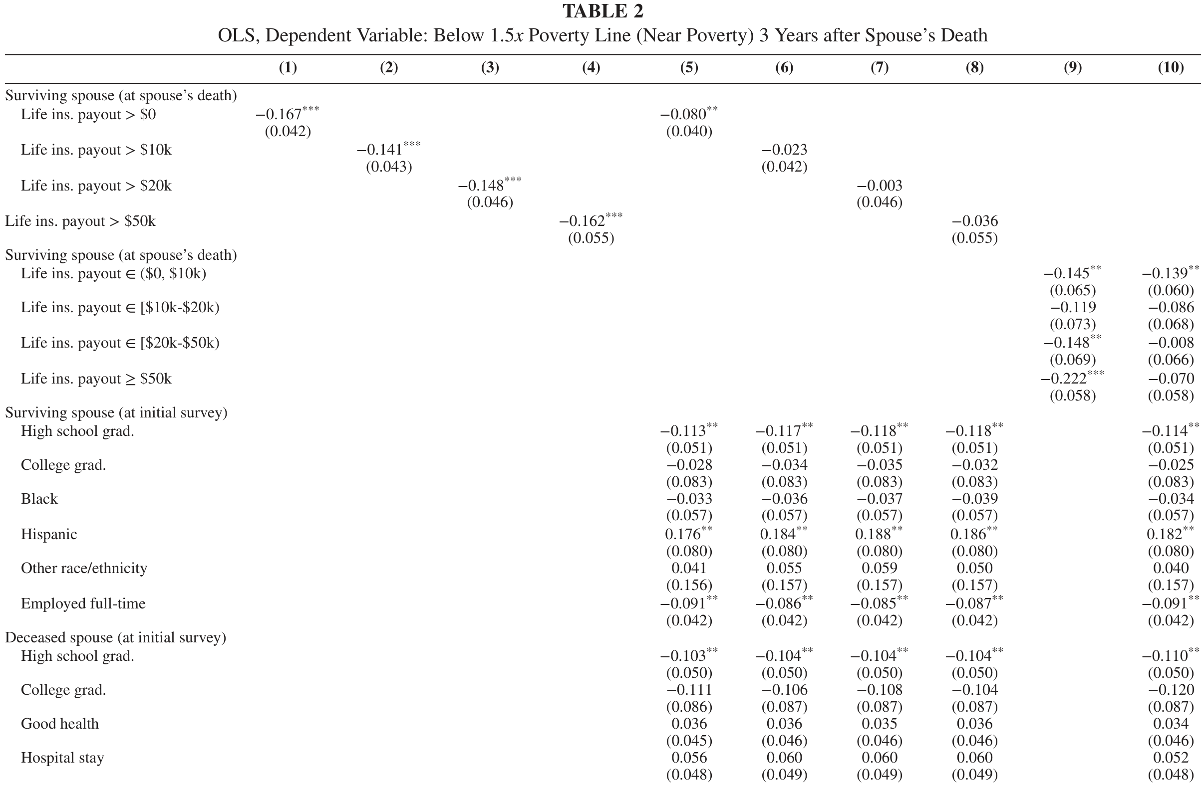
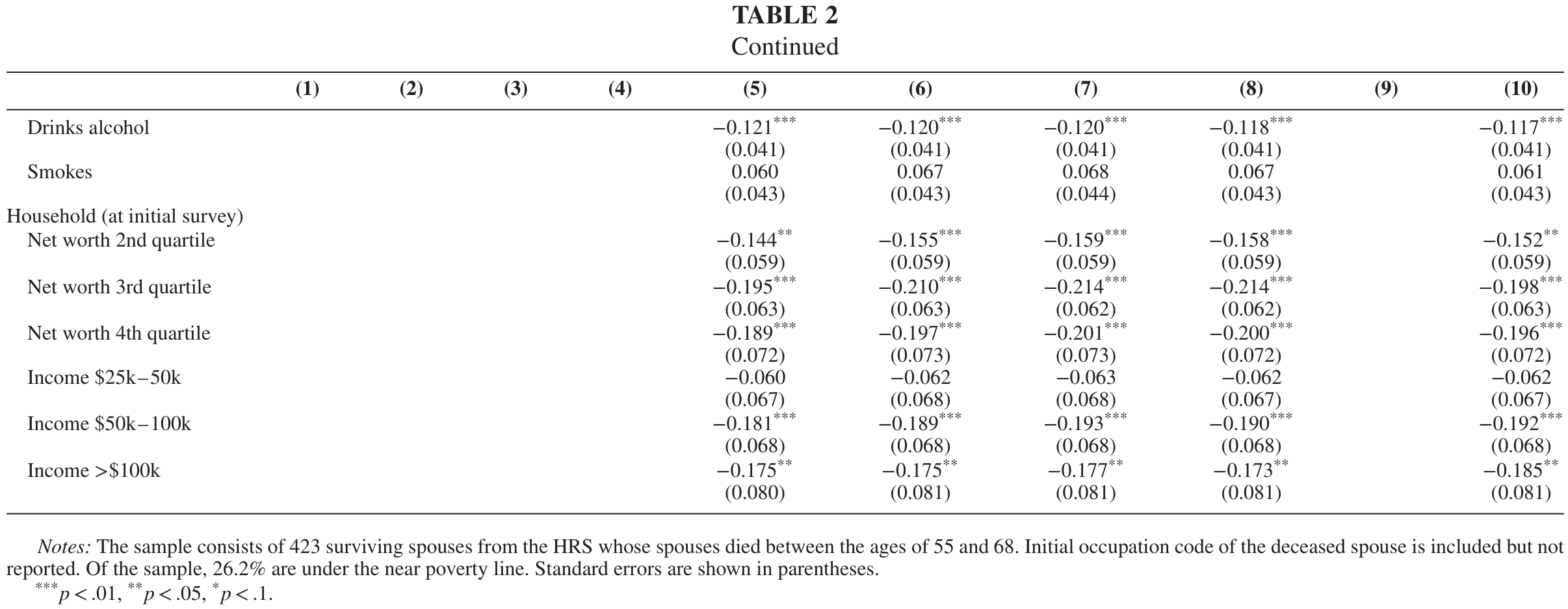
To give a baseline comparison, we first regress having income below 1.5 _x_ FPL on receiving a payout without controls. The first columns of Table 2 show a significant correlation between receiving a payout and being above the 1.5 _x_ FPL and that larger payouts lead to greater reductions in the likelihood of being below 1.5 _x_ FPL. Column 5 shows that after the inclusion of controls, the effect is drastically reduced from 16.7 to 8.0 percentage points less likely to be under 1.5 _x_ FPL due to receiving a payout from a base of 26.2%. Additionally, with the inclusion of covariates the effect of larger payouts becomes insignificant as shown in columns 6–8.

### Figure 1. CDF: Life Insurance Payouts

<figure class="article-figure" id="figure-1"><a href="/files/publications/ay-ja-jedvw72pczhlfo32-assets/figure-1.png"><img alt="Figure 1. Cumulative distribution of life insurance payouts among recipients whose spouses died at ages 55–68 in the Health and Retirement Study; the horizontal axis shows payout dollars and the vertical axis the cumulative share." height="852" loading="lazy" src="/files/publications/ay-ja-jedvw72pczhlfo32-assets/figure-1.png" width="788"/></a><figcaption>Figure 1. <a href="/files/publications/ay-ja-jedvw72pczhlfo32-assets/figure-1.png">Open full-resolution image</a>.</figcaption></figure>


The final two columns help illustrate the influence of various levels of coverage. Consistent with the previous findings, column 9 shows that as the payout increases, the likelihood of being under 1.5 _x_ FPL decreases. The last column shows that after controlling for socioeconomic status, life insurance payouts over $10,000 have no statistically significant influence on the well-being of the surviving spouse. Given that we do not find an effect 3 years following the spouse’s death, it is very unlikely that we would find a significant effect looking at a longer time horizon.<sup><a href="#source-note-11" aria-label="Source note 11">11</a></sup> However, for life insurance payouts less than $10,000, the coefficient’s magnitude does not significantly change with controls and remains statistically significant implying that receiving a payout less than $10,000 causes a 13.9 percentage point
reduction in the likelihood of being below the near poverty line.

A priori, one might not expect small payouts to significantly influence well-being. One possible explanation for the persistence of the statistically significant result is that the small payouts largely represent basic ESLI coverage that is automatically provided by an employer. The HRS does not distinguish between ESLI and individual market payouts. Nonetheless, term life insurance policies are generally sold starting at $25,000 or $50,000, which means that individuals that received payouts of less than $10,000 likely did not have individual term coverage.<sup><a href="#source-note-12" aria-label="Source note 12">12</a></sup> If these small payouts originated from basic ESLI coverage rather than individual market coverage, then the payouts are not the result of active financial planning. These small payments or “death benefits” potentially increase well-being through the reduction of costly financial choices including using payday loans, or carrying balances on credit cards to deal with the immediate financial costs following the death of a spouse for individuals who presumably did not avail themselves of more rigorous individual market coverage.

### Table 2. OLS, Dependent Variable: Below 1.5x Poverty Line (Near Poverty) 3 Years after Spouse’s Death

<figure class="article-figure" id="table-2-part-1"><a href="/files/publications/ay-ja-jedvw72pczhlfo32-assets/table-2-part-1.png"><img alt="Table 2, first panel. Ten ordinary least squares specifications for near poverty three years after a spouse's death, with life-insurance payout thresholds or ranges and surviving and deceased spouse characteristics." height="1584" loading="lazy" src="/files/publications/ay-ja-jedvw72pczhlfo32-assets/table-2-part-1.png" width="2412"/></a><figcaption>Table 2, first page. <a href="/files/publications/ay-ja-jedvw72pczhlfo32-assets/table-2-part-1.png">Open full-resolution image</a>.</figcaption></figure>
<figure class="article-figure" id="table-2-part-2"><a href="/files/publications/ay-ja-jedvw72pczhlfo32-assets/table-2-part-2.png"><img alt="Table 2, continuation. Remaining health, household wealth and income coefficients for the ten near-poverty models, with sample and statistical-significance notes." height="936" loading="lazy" src="/files/publications/ay-ja-jedvw72pczhlfo32-assets/table-2-part-2.png" width="2412"/></a><figcaption>Table 2, continued. <a href="/files/publications/ay-ja-jedvw72pczhlfo32-assets/table-2-part-2.png">Open full-resolution image</a>.</figcaption></figure>


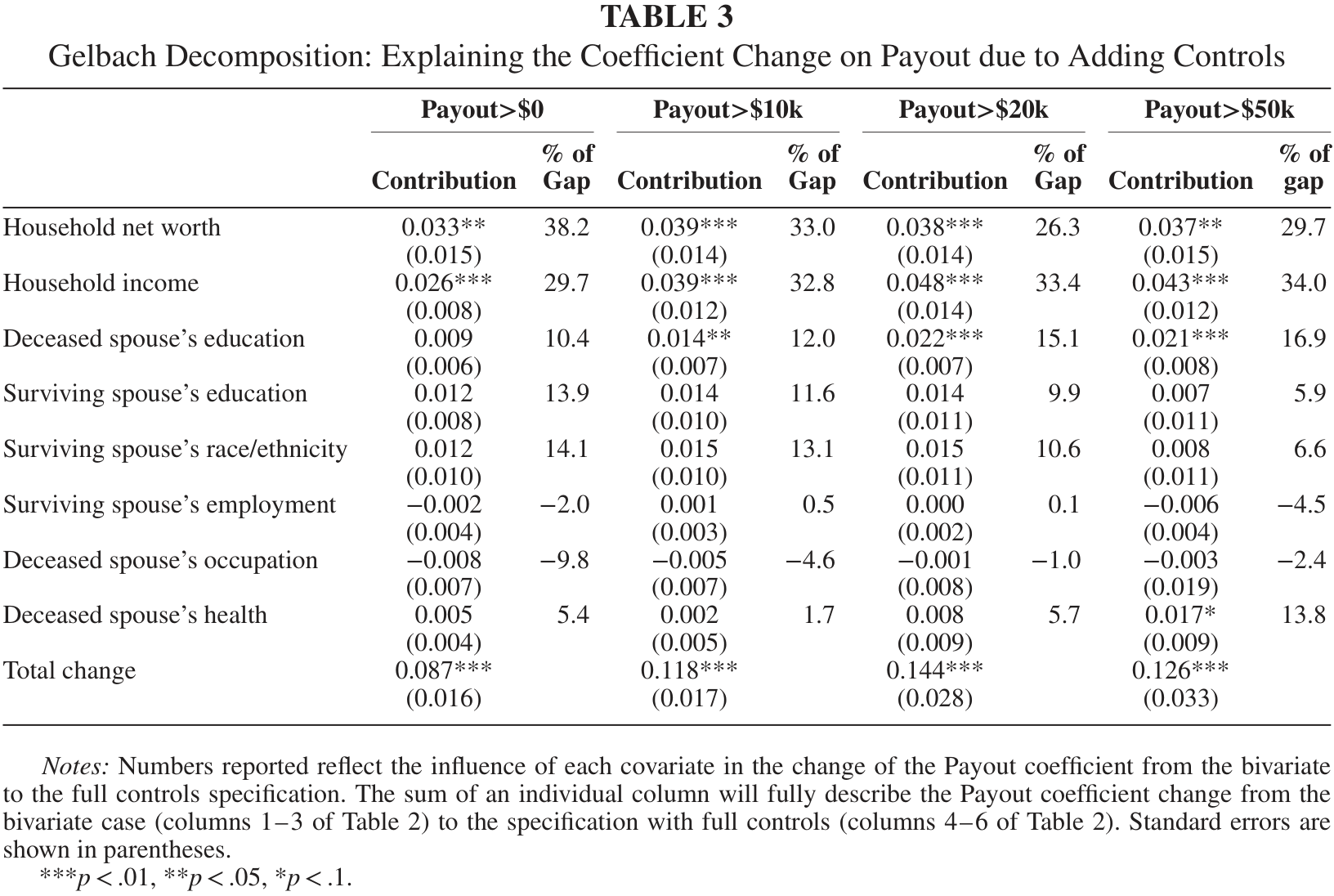
To understand which covariates cause the change in magnitude from the regression without controls to the full specification with controls we use a decomposition method described in Gelbach (2016). Essentially, the traditional method of sequentially adding covariates to see changes in the coefficient of interest produces ambiguous results based on the order in which covariates are added. Gelbach (2016) proposes calculating the omitted variable bias of excluding each covariate separately from the full model to ascertain the contribution of each covariate to the total change. Table 3 illustrates the influence of different groups of controls in explaining the percentage point change in the coefficient for <math xmlns="http://www.w3.org/1998/Math/MathML" display="inline"><mrow><mi>T</mi><mi>o</mi><mi>t</mi><mi>a</mi><mi>l</mi><mtext>&#x000A0;</mtext><mi>P</mi><mi>a</mi><mi>y</mi><mi>o</mi><mi>u</mi><msub><mi>t</mi><mi>i</mi></msub></mrow></math>. For example, isolating the regressions that use receiving any payout as the independent variable of interest (columns 1 and 5 of Table 2) the total change in the coefficient from adding controls was 0.087 (from −0.167 to −0.080). Table 3 demonstrates that 38.2% of the change in the coefficient on receiving a payout comes from controlling for household net worth. As well, the addition of household income accounts for 29.7% of the overall coefficient change from adding covariates. This reflects not only the correlation of net worth and income with the well-being of the surviving spouse, but also the correlation between these factors and receiving a payout. Overall, about 60–65% of the change in the coefficients for the payouts can be attributed to net worth and household income. This table also shows that the deceased spouse’s education becomes increasingly important as the payout threshold increases in explaining the decrease in influence of life insurance payouts. These findings illustrate that a majority of the effect of life insurance payouts is likely due to financial acumen as captured by net worth, income and the deceased spouse’s education. This finding is consistent with the results of Lusardi, Michaud, and Mitchell (Forthcoming) who show that 30–40% of retirement wealth inequality comes from differences in financial knowledge.

### Table 3. Gelbach Decomposition: Explaining the Coefficient Change on Payout due to Adding Controls

<figure class="article-figure" id="table-3"><a href="/files/publications/ay-ja-jedvw72pczhlfo32-assets/table-3.png"><img alt="Table 3. Gelbach decomposition of the change in the payout coefficient after adding controls, showing contributions and percentages of the gap from wealth, income, education, race, employment, occupation and health." height="1096" loading="lazy" src="/files/publications/ay-ja-jedvw72pczhlfo32-assets/table-3.png" width="1632"/></a><figcaption>Table 3. <a href="/files/publications/ay-ja-jedvw72pczhlfo32-assets/table-3.png">Open full-resolution image</a>.</figcaption></figure>


Notwithstanding these results for larger payouts, one would expect that receiving $50,000 could have a measurable influence on financial well-being even after controlling for socioeconomic status. One possible explanation for the lack of a significant effect of life insurance on the well-being of surviving spouses is that individuals spend the money soon after receipt rather than using it to replace lost future income. There is ample evidence supporting this argument. A similar type of lump sum distribution occurs when individuals with defined contribution (DC) plans change employment. When employees switch
jobs, they generally have the option to leave their DC pension plans with their former employer, rollover the amount into their new employers’ DC plan, or receive a preretirement lump sum distribution. Poterba and Venti (1998) find that lump sum distributions are common and most distributions are not rolled over into qualified retirement saving accounts. In order to encourage rollover of lump sum distributions into qualified savings accounts—rather than increase spending from the distribution—the federal government implemented excise taxes and withholding taxes to discourage such behavior. Chang (1996) finds that such tax penalties in general encourage rollover into qualified savings accounts but do not significantly deter the use of funds for current consumption by lower-income recipients. In addition, Johnson, Parker,
and Souleles (2006) in a study on tax rebate spending find that individuals with the lowest income and the least liquid assets—those that are most likely to be near the poverty line—spent significantly more of the rebate relative to higher income individuals. This persistent tendency to quickly spend lump sum transfers, especially for those that are close to the poverty line, certainly could be the reason that medium- or long-run outcomes are unaffected.


One possible alternative to lump sum distributions of life insurance payouts is annuitization. It is likely that sophisticated financial planning, like annuitization, is a low priority given the circumstances surrounding a premature or unexpected death. In the context of lump sum payments from DC plans, Brown (2009) argues for automatic annuitization to provide a guaranteed income stream for life to hedge against the risk of outliving one’s assets. Furthermore, Bütler and Teppa (2007) show using Swiss data that an initial default of annuitization is effective at increasing overall annuitization.

The literature on behavioral economics potentially sheds light on policy options to make lump sum payments from life insurance more effective. Individuals tend to display time inconsistent preferences thus necessitating the need for commitment mechanisms (Laibson 1997). Research has shown that individuals display relatively high discount rates in the short run, but lower discount rates in the long run known as hyperbolic discounting (Ainslie 1992). Therefore, households would be more likely to sign on to annuitization of life insurance payouts at the time they purchase life insurance coverage than at the time of the payout. Additionally, inertia in financial decisions decreases the likelihood that individuals would change the initial selection (Madrian and Shea 2001; Chetty et al. 2014; Harris and Yelowitz 2016). Consequently, an initial
default of annuitization of ESLI payouts (with the possibility of opting into a lump sum payment) might circumvent the issue of increased consumption following a large life insurance payout.

However, there is one possible concern with automatic annuitization of life insurance payouts. Due to correlated socioeconomic status and bereavement effects, life expectancy between a husband and wife is highly correlated (Espinosa and Evans 2008). The value of a life annuity is directly related to the owner’s longevity and longer-lived individuals have more to gain from an annuity relative to shorter-lived individuals. Consequently, annuities would be a relatively worse deal for surviving spouses who have a higher mortality rate than the typical annuitant. Nonetheless, if insurance companies used pooled life insurance payout recipients in the determination of annuity payments then bundling the two products could be advantageous.
### B. Additional Metrics of Well-being
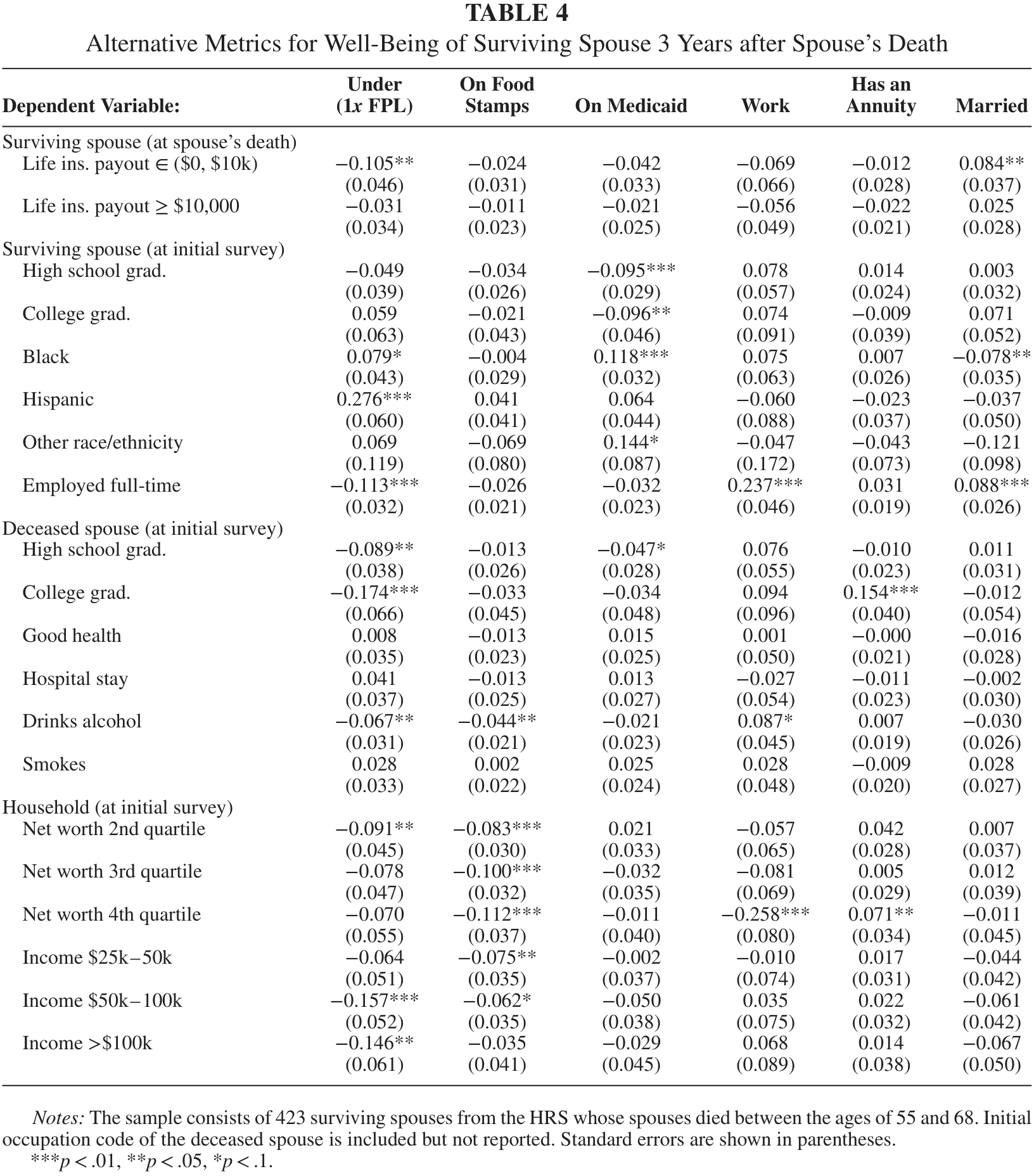
Given the somewhat arbitrary nature of the cutoff of 1.5 _x_ FPL, we include alternative metrics for the well-being of a surviving spouse presented in Table 4. The first column shows that the finding for being under the poverty line is consistent with the analysis discussed above for being under the near poverty line. The subsequent columns show that after controlling for covariates, there is no statistically significant influence on other metrics of widow well-being such as food stamp participation and Medicaid coverage. In addition, life insurance payouts have the potential to decrease other, arguably less-efficient, ways of smoothing consumption such as increased labor force participation and remarriage. Table 4 further shows that receiving a life insurance payout does not reduce labor supply or remarriage. Additionally, the table shows that receiving a life insurance payout does not increase annuitization, providing support that individuals do not use annuities to smooth consumption after receiving a lump-sum transfer as previously discussed.

### Table 4. Alternative Metrics for Well-Being of Surviving Spouse 3 Years after Spouse’s Death

<figure class="article-figure" id="table-4"><a href="/files/publications/ay-ja-jedvw72pczhlfo32-assets/table-4.png"><img alt="Table 4. Estimates for six alternative measures of surviving-spouse well-being three years after death: poverty, food stamps, Medicaid, work, annuity ownership and marriage, with payout and demographic coefficients." height="1856" loading="lazy" src="/files/publications/ay-ja-jedvw72pczhlfo32-assets/table-4.png" width="1632"/></a><figcaption>Table 4. <a href="/files/publications/ay-ja-jedvw72pczhlfo32-assets/table-4.png">Open full-resolution image</a>.</figcaption></figure>


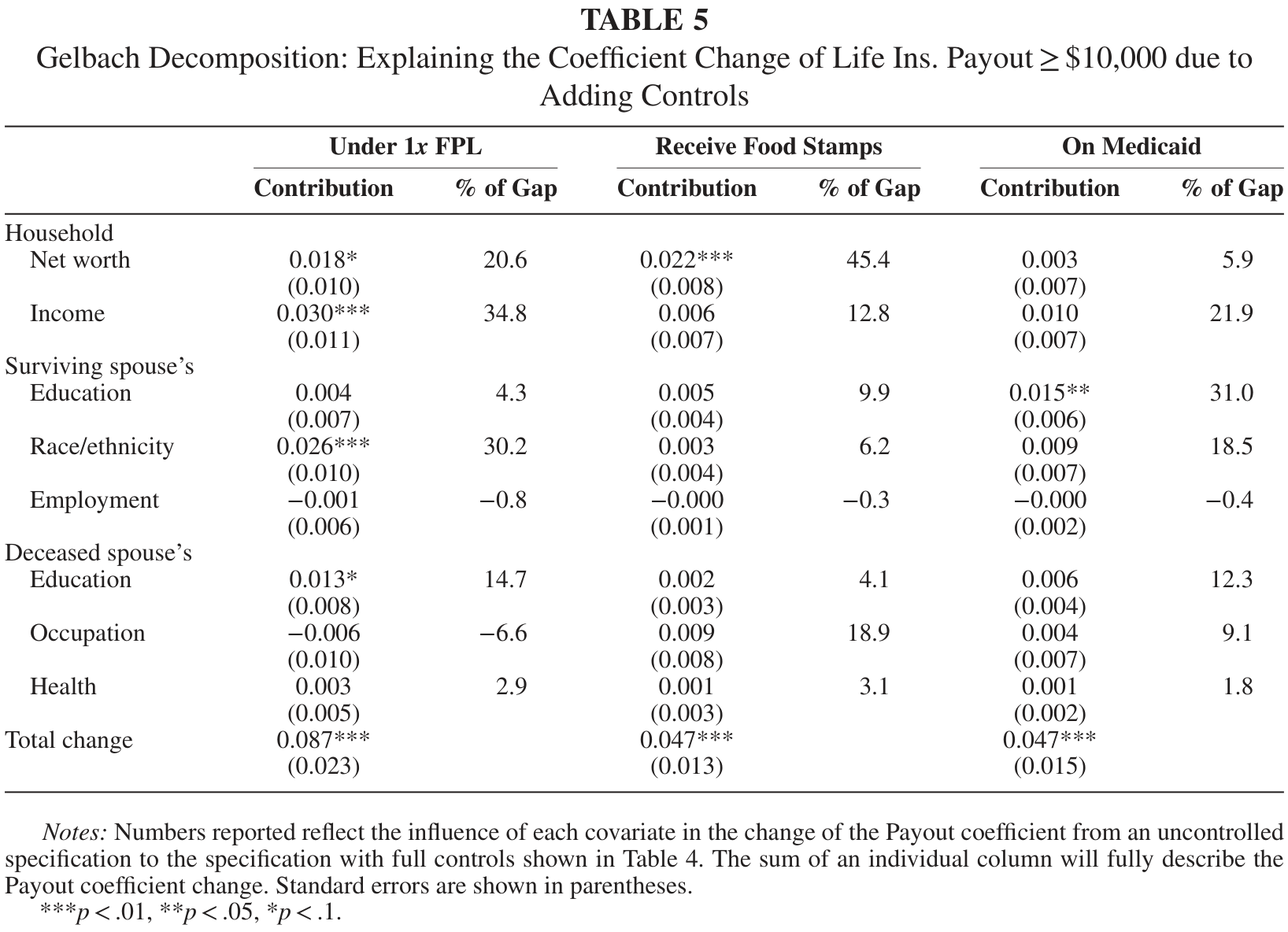
Once again, to see the cause for the statistically insignificant results for payouts we present the Gelbach Decomposition of the coefficient on payouts greater than $10,000 for the first three metrics, which significantly changed due to the addition of covariates.<sup><a href="#source-note-13" aria-label="Source note 13">13</a></sup> Table 5 shows that household net worth and income account for the majority of the change for the specification that uses being under the poverty line as the dependent variable. Ethnic and racial differences also play an important role in the reduction of the coefficient’s magnitude reflecting correlation between poverty and race/ethnicity as well as a correlation between race/ethnicity and receiving a life insurance payout. The most important covariate in describing the decrease in the effect of payouts on Medicaid participation is the education of the surviving spouse, which accounts for 31.0% of the total change.

### Table 5. Gelbach Decomposition: Explaining the Coefficient Change of Life Ins. Payout≥ $10,000 due to Adding Controls

<figure class="article-figure" id="table-5"><a href="/files/publications/ay-ja-jedvw72pczhlfo32-assets/table-5.png"><img alt="Table 5. Gelbach decomposition for payouts of at least $10,000 in models of poverty, food stamps and Medicaid, reporting each control group's contribution and share of the coefficient change." height="1184" loading="lazy" src="/files/publications/ay-ja-jedvw72pczhlfo32-assets/table-5.png" width="1636"/></a><figcaption>Table 5. <a href="/files/publications/ay-ja-jedvw72pczhlfo32-assets/table-5.png">Open full-resolution image</a>.</figcaption></figure>


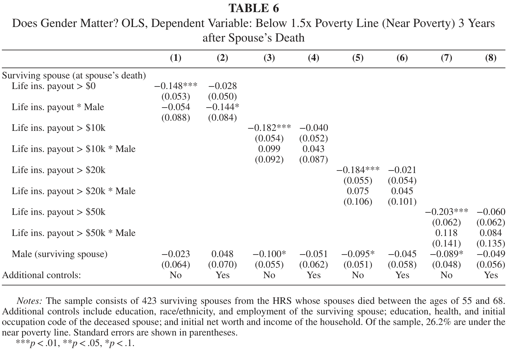
Lastly, in Table 6 we show that the effect of life insurance payouts is essentially the same for widows and widowers. The one exception is that receiving any payout has a slightly greater influence on surviving men relative to women.

### Table 6. Does Gender Matter? OLS, Dependent Variable: Below 1.5x Poverty Line (Near Poverty) 3 Years after Spouse’s Death

<figure class="article-figure" id="table-6"><a href="/files/publications/ay-ja-jedvw72pczhlfo32-assets/table-6.png"><img alt="Table 6. Eight near-poverty regression specifications with life-insurance payout thresholds, male-survivor interactions and models with or without additional controls, including standard errors and full sample notes." height="1132" loading="lazy" src="/files/publications/ay-ja-jedvw72pczhlfo32-assets/table-6.png" width="1636"/></a><figcaption>Table 6. <a href="/files/publications/ay-ja-jedvw72pczhlfo32-assets/table-6.png">Open full-resolution image</a>.</figcaption></figure>


## VI. CONCLUSION
Premature death of a breadwinner can have devastating financial consequences on the surviving spouse. Increased longevity and years spent in retirement for the surviving spouse only exacerbates these negative consequences. Additionally, the aging population in the United States is straining the Social Security System including Survivor’s Benefits, which provided an average monthly benefit of $1,309 to 3.8 million widows and widowers in 2010 (Shelton and Nuschler 2012). These features highlight the importance of life insurance in mitigating the negative financial consequences of premature death on elderly surviving spouses. Not only could life insurance reduce these negative financial consequences, but it also has the potential of reducing dependence on other government assistance programs such as SNAP, Medicaid, and SSI for elderly surviving spouses.

Using the HRS, we analyze the effect of life insurance coverage and subsequent payouts on the well-being of surviving spouses. We find that after controlling for financial and educational factors, the influence of life insurance payouts greater than $10,000 disappears. These findings indicate that larger life insurance payouts are more of a marker for financial planning rather than a driver at improving the well-being of surviving spouses and decreasing the incidence of government assistance. For smaller payouts, we find a significant influence on the well-being of surviving spouses that likely originated from basic ESLI automatically provided by the employer. This result points to the potential role of basic ESLI coverage at improving the well-being of surviving spouses. Nonetheless, the HRS does not distinguish between ESLI and individual market payouts making the source of the significance less concrete. The HRS is the only panel dataset of which we are aware that allows us to follow a reasonably sized sample of widows and widowers before and after the death of their spouse and also observe life insurance payouts. Nevertheless, our sample sizes are fairly small.

 A natural question that remains, given that well-being is unaffected by large payouts, is how are lump-sum life insurance payouts actually utilized? Evidence from other studies suggests different lump sum payments translate into immediate, increased consumption but no parallel evidence exists for life insurance payouts.

 Assuming that behavior from life insurance payouts is in fact similar, a potential way to increase the effectiveness of life insurance is through a restructuring of policies for ESLI. Employers in conjunction with insurance companies could structure policies such that annuitization was the default method of receiving payout rather than a lump sum transfer. Given the extensive literature on inertia in the workplace, it is likely that relatively few employees would opt out of default annuitization of life insurance payouts for their dependents, thereby potentially increasing well-being of surviving spouses.

 Another question that arises from these findings is how large would life insurance payouts need to be to significantly influence well-being of surviving spouses. From our analysis, we know that even $50,000 payouts do not significantly change the well-being of surviving spouses. This implies that payouts would need to be larger, but how large it would need to be is uncertain, and without annuitization, it is unclear whether larger payouts would significantly influence well-being.

## References
- Ainslie, G. _Picoeconomics_ . Cambridge: Cambridge University Press, 1992.
- American Council of Life Insurers. 2015. “2015 Life Insurance Fact Book.” https://www.acli.com/Tools/Industry%20Facts/Life%20Insurers%20Fact%20Book/Documents/FB15All.pdf.
- Angrist, J. D. “Lifetime Earnings and the Vietnam Era Draft Lottery: Evidence from Social Security Administrative Records.” _American Economic Review_ , 80(3), 1990, 313–36.
- Angrist, J. D., and J. Pischke. _Mostly Harmless Econometrics: An Empiricist’s Companion_ , Vol. 1. Princeton, NJ: Princeton University Press, 2009.
- Auerbach, A. J., and L. J. Kotlikoff. “The Adequacy of Life Insurance Purchases.” _Journal of Financial Intermediation_ , 1(3), 1991, 215–41.
- Bellet, A. Z. “Employer-sponsored Life Insurance: A New Look.” _Monthly Labor Review_ , 112(10), 1989, 25–28.
- Bernheim, B. D., L. Forni, J. Gokhale, and L. J. Kotlikoff. “The Mismatch between Life Insurance Holdings and Financial Vulnerabilities: Evidence from the Health and Retirement Study.” _American Economic Review_ , 93(1), 2003, 354–65.
- Brown, J. R. 2009. “Automatic Lifetime Income as a Path to Retirement Income Security.” Washington, DC: American Council of Life Insurers.
- Browne, M. J., and K. Kim. “An International Analysis of Life Insurance Demand.” _Journal of Risk and Insurance_ , 60(4), 1993, 616–34.
- Bütler, M., and F. Teppa. “The Choice between an Annuity and a Lump Sum: Results from Swiss Pension Funds.” _Journal of Public Economics_ , 91(10), 2007, 1944–66.
- Chang, A. E. “Tax Policy, Lump-sum Pension Distributions, and Household Saving.” _National Tax Journal_ , 49(2), 1996, 235–52.
- Chetty, R., J. N. Friedman, S. Leth-Petersen, T. H. Nielsen, and T. Olsen. “Active vs. Passive Decisions and Crowd-Out in Retirement Savings Accounts: Evidence from Denmark.” _Quarterly Journal of Economics_ , 129(3), 2014, 1141–219.
- Cseh, A. “The Effects of Depressive Symptoms on Earnings.” _Southern Economic Journal_ , 75(2), 2008, 383–409.
- Currie, J., and A. Yelowitz. “Are Public Housing Projects Good for Kids?” _Journal of Public Economics_ , 75(1), 2000, 99–124.
- Elliott, D. B., and T. Simmons. “Marital Events of Americans: 2009.” American Community Survey Reports. Washington, DC: US Department of Commerce, Economics and Statistics Administration, US Census Bureau, 2011.
- Espinosa, J., and W. N. Evans. “Heightened Mortality after the Death of a Spouse: Marriage Protection or Marriage Selection?” _Journal of Health Economics_ , 27(5), 2008, 1326–42.
- Fadlon, I., and T. H. Nielsen. “Household Responses to Severe Health Shocks and the Design of Social Insurance.” NBER Working Paper No. 21352, 2015. Accessed October 26, 2016. http://www.nber.org/papers/w21352.pdf.
- Gandolfi, A. S., and L. Miners. “Gender-Based Differences in Life Insurance Ownership.” _Journal of Risk and Insurance_ , 63(4), 1996, 683–93.
- Gelbach, J. B. “When Do Covariates Matter? And Which Ones, and How Much?” _Journal of Labor Economics_ , 34(2), 2016, 509–43.
- Grogger, J. “The Effect of Arrests on the Employment and Earnings of Young Men.” _Quarterly Journal of Economics_ , 110(1), 1995, 51–71.
- Grossman, G. M. “Life Insurance Benefits in Small Establishments and Government.” _Monthly Labor Review_ , 115, 1992, 33–36.


- Harris, T. F., and A. Yelowitz. “Nudging Life Insurance in the Workplace.” _Economic Inquiry_ , Epub 2016 Sep 6. doi: 10.1111/ecin.12390.
- Horrace, W. C., and R. L. Oaxaca. “Results on the Bias and Inconsistency of Ordinary Least Squares for the Linear Probability Model.” _Economics Letters_ , 90(3), 2006, 321–27.
- Hotz, V. J., S. W. McElroy, and S. G. Sanders. “Teenage Childbearing and Its Life Cycle Consequences: Exploiting a Natural Experiment.” _Journal of Human Resources_ , 40(3), 2005, 683–715.
- Johnson, D. S., J. A. Parker, and N. S. Souleles. “Household Expenditure and the Income Tax Rebates of 2001.” _American Economic Review_ , 96(5), 2006, 1589–610.
- Laibson, D. “Golden Eggs and Hyperbolic Discounting.” _Quarterly Journal of Economics_ , 112(2), 1997, 443–77.
- Lusardi, A., P.-C. Michaud, and O. S. Mitchell. “Optimal Financial Knowledge and Wealth Inequality.” _Journal of Political Economy_ , Forthcoming.
- Madrian, B. C., and D. F. Shea. “The Power of Suggestion: Inertia in 401(k) Participation and Savings Behavior.” _Quarterly Journal of Economics_ , 116(4), 2001, 1149–87.
- Neumark, D. “Age Discrimination Legislation in the United States.” _Contemporary Economic Policy_ , 21(3), 2003, 297–317.
- Poterba, J. M., and S. F. Venti. “Lump-sum Distributions from Retirement Saving Plans: Receipt and Utilization,” in _Inquiries in the Economics of Aging_ , edited by D. A. Wise. Chicago: University of Chicago Press, 1998, 85–108.
- Rees, D. I., L. M. Argys, and S. L. Averett. “New Evidence on the Relationship between Substance Use and Adolescent Sexual behavior.” _Journal of Health Economics_ , 20(5), 2001, 835–45.
- Sevak, P., D. R. Weir, and R. J. Willis. “The Economic Consequences of a Husband’s Death: Evidence from the HRS and AHEAD.” _Social Security Bulletin_ , 65(3), 2004, 31–44.
- Shelton, A. M., and D. Nuschler. “Social Security: Revisiting Benefits for Spouses and Survivors.” Washington, DC: Congressional Research Service, 2012. Accessed October 26, 2016. http://greenbook.waysandmeans.house.gov/sites/greenbook.waysandmeans.house.gov/files/2012/documents/R41479_gb_1.pdf.
- U.S. Department of Labor. “National Compensation Survey: Employee Benefits in the United States, March 2015.” 2015. Accessed October 26, 2016. http://www.bls.gov/ncs/ebs/benefits/2015/ebbl0057.pdf.

## Notes

<p id="source-note-1"><strong>1.</strong> Percentages calculated from tabulations of the 1990, 1991, 1992, and 1993 panels of the Survey of Income and Program Participation (SIPP) using individual weights.</p>

<p id="source-note-2"><strong>2.</strong> Average level of basic coverage calculated from the Employee Benefits Survey for private firms and the March 2015 National Compensation Survey.</p>

<p id="source-note-3"><strong>3.</strong> The Age Discrimination in Employment Act (ADEA) prevents employers from discriminating against older workers in benefits. However, if employers spend equal amounts to buy life insurance coverage for old and young employees, they do not violate the ADEA even though this translates into more coverage for the young. For a review of the ADEA see Neumark (2003).</p>

<p id="source-note-4"><strong>4.</strong> The RAND version imputes income and assets based on unfolding bracket questions that are used in this study. For full documentation see http://hrsonline.isr.umich.edu/modules/meta/rand/randhrso/randhrs_O.pdf</p>

<p id="source-note-5"><strong>5.</strong> Given the biennial nature of the HRS, we technically look at the financial status of individuals 2 to 3 years following their spouse’s death. For brevity, in the text we simply refer to this as 3 years.</p>

<p id="source-note-6"><strong>6.</strong> Life expectancy estimates come from the Social Security Administration Period Life Table, 1994. See https://web.archive.org/web/19970617031009/http://www.ssa.gov/OACT/STATS/table4c6.html.</p>

<p id="source-note-7"><strong>7.</strong> All dollar amounts are converted to 2012 dollars using the Consumer Price Index.</p>

<p id="source-note-8"><strong>8.</strong> We use the RAND measure of total household income less food stamp income for income used in the poverty status calculations. A more accurate measure would add income from all non-core household residents to the measure of total household income. However, for earlier years in the sample, income from non-core household residents is not available. Consequently, we use official poverty thresholds for the relevant years from the Bureau of Labor Statistics (BLS) and assume that the household contains only the individual after the death of the spouse. In addition, the thresholds given by the BLS have discontinuities at age 65, which could confound our analysis. We therefore use the threshold for those under 65 regardless of age.</p>

<p id="source-note-9"><strong>9.</strong> Advantages of the linear probability model are discussed in Angrist and Pischke (2009). For the main specifications, more than 85% of the predicted values lie within the 0/1 interval, reducing the potential bias of using the linear probability model (Horrace and Oaxaca 2006). The main results from the linear probability specifications are consistent with estimated probit model results.</p>

<p id="source-note-10"><strong>10.</strong> Gandolfi and Miners (1996) find that education increases life insurance holdings and Browne and Kim (1993) postulate that a higher education level raises life insurance holdings through increased risk aversion and awareness of the necessity of insurance.</p>

<p id="source-note-11"><strong>11.</strong> Due to sample size limitations, we do not look at longer time horizons than 3 years.</p>

<p id="source-note-12"><strong>12.</strong> See www.quickquote.com and www.term4sale.com for examples of commonly available policies.</p>

<p id="source-note-13"><strong>13.</strong> The coefficients on payouts larger than $10,000 do not significantly change from the controlled to uncontrolled regressions using working, annuities, and marital status as the dependent variable. Consequently, a decomposition is uninformative.</p>