Complete article reading edition. Tables and figures reproduce the published source; open an image for full resolution. The PDF retains the original page layout.
## Abstract
This article assesses the importance of receiving supplemental health insurance on participation in Supplemental Security Income (SSI) for the elderly. The implementation of the Qualified Medicare Beneficiary (QMB) program offered a substitute for Medicaid, and expanded health insurance eligibility to a higher income level. Using a sample of elderly respondents aged 66 to 75, I find that the QMB program reduced SSI participation. More than half of the QMB participants were previously covered by SSI and Medicaid. The calculations suggest that the QMB program was not as expensive as it might first appear because of reductions in SSI expenditure.
**JEL classification:** H53; I38; J14
**Author note:** I am grateful to Janet Currie, David Cutler, Leora Friedberg, Jonathan Gruber, Joseph Hotz, Wei-Yin Hu, Kevin Murphy, James Poterba, Duncan Thomas, Robert Topel, Lori Yelowitz, two anonymous referees, and the editor for helpful suggestions; to John Beauchamp, Gloria Chiang, Ida Kulukian, Thong Ly, and Sheri Zwirlein for excellent research assistance; and to participants at the University of Chicago and NBER Health Economics seminar. This research was supported by the UCLA Academic Senate and the NBER Health and Aging Fellowship. The data and computer programs used in this study are available from the author.
**Author contact:** Aaron S. Yelowitz, Assistant Professor, Department of Economics, University of California, Los Angeles, CA 90095. Phone: 1-310-825-5665; Fax: 1-310-825-9528; E-mail: yelowitz@ucla.edu.
**Abbreviations:** AIME, Average Indexed Monthly Earnings; AFDC, Aid to Families with Dependent Children; CPS, Current Population Survey; MCCA, Medicare Catastrophic Coverage Act; MN, Medically Needy; OBRA, Omnibus Reconciliation Act; QMB, Qualified Medicare Beneficiary; SIPP, Survey of Income and Program Participation; SLMB, Specified Low-Income Medicare Beneficiaries; SSA, Social Security Administration; SSI, Supplemental Security Income.
## I. INTRODUCTION
The Supplemental Security Income (SSI) program in the United States provides assistance to elderly, blind, and disabled individuals who are poor. It is federally financed and administered by the Social Security Administration. Although much more attention has been focused on the former Aid to Families with Dependent Children (AFDC) program, which primarily targets poor single-parent families, more money was spent on cash relief for SSI recipients in 1993: $23.6 billion compared to $22.3 billion.1 In addition to cash, SSI recipients receive supplemental health insurance coverage for Medicare, similar to private Medigap policies, through the Medicaid program. This provides a second important benefit to SSI recipients: in fiscal year 1993, Medicaid expenditure for elderly, categorically needy SSI recipients amounted to $14.1 billion.2
Several studies have examined the importance of health insurance for working-age adults in the labor market.3 In addition, the effects of recent Medicaid expansions for younger populations have been extensively studied.4 Little is known, however, about the quantitative importance of Medicaid on the SSI participation of the elderly. The key obstacle in assessing this effect is that, until recently, Medicaid eligibility had been closely related to SSI eligibility in most states. This study analyzes the introduction of the Qualified Medicare Beneficiary (QMB) program, enacted in different states from 1987 to 1992, which offered supplemental health insurance coverage to the elderly without the need to participate in SSI. The QMB program offered some of the same Medicare cost sharing benefits that an elderly SSI recipient would receive from Medicaid, including the payment of Medicare premiums, deductibles, and copayments.5 Moreover, the QMB program expanded Medicaid coverage to individuals with higher incomes and assets than the SSI program.6
The primary goal of this article is to document the link between the QMB program and the decision to participate in SSI. I find that raising the income limit in QMB program significantly reduces SSI participation, particularly among African-Americans and the less educated. The coefficient estimates suggest that, in the absence of the QMB buy-in program, SSI participation would have been 45% higher in 1992 than it actually was. The caseload growth in the elderly SSI population would have looked very similar to the caseload growth of the disabled SSI population, a group not eligible for QMB. In addition, the QMB program was considerably less expensive than one would infer from simply calculating the increased health care expenditure because of reductions in SSI expenditure for cash benefits.
The rest of the article is arranged as follows. Section II outlines some relevant features of the SSI, Medicaid, and QMB programs. In particular, it reviews how the income eligibility limits for QMB and SSI are computed. The difference between those limits is a measure of how closely are Medicaid and SSI linked. It will subsequently be used as the key independent variable in the regression analysis. This section also shows the cross-sectional and time-series variation in the QMB program. Section III models the potential effects on SSI participation of the introduction of the QMB program, and considers the role of information. By providing an alternative source of health insurance, the QMB program might reduce SSI participation. But if QMB increases awareness about other transfer programs to the elderly, then it could increase SSI participation. Section IV provides a data description. I use repeated cross sections of the March Current Population Survey from the calendar years 1987 to 1992—the period when the QMB expansions were being phased in. Section V presents the empirical results and cost implications. Section VI concludes.
## II. BACKGROUND ON THE SSI, MEDICAID, AND QMB PROGRAMS
### The SSI Program
The federal government introduced the Supplemental Security Income (SSI) program in 1974. It replaced old-age assistance programs previously run by the states. In 1994, SSI paid an annual maximum benefit of $5,352 to an individual and $8,028 to a couple. In addition, roughly half of the states supplement the federal SSI benefit. In 1994, the median state supplement (conditional on providing a supplement) was $468 per year to a couple, though the supplement exceeded $1,200 in several states.
To be eligible for SSI, the recipient’s annual income must be less than a state-specific limit.7 This limit, in turn, will be vital in determining how much the budget constraint changes from the QMB laws, and in constructing a sensible independent variable in the regression analysis. If all of an individual’s income is in the form of nonwage income, then the SSI limit is determined as:
**Equation (1):**
where is the maximum annual income for SSI eligibility, and represent the federal and state annual SSI grant for a recipient with zero income, and represents the annual standard deduction (equal to $240).
If all of the individual’s income is in the form of wages, then the limit is:
**Equation (2):**
where represents the benefit reduction rate (equal to 50%), represents an annual work expense deduction (equal to $780), and the other variables are as defined above. An individual in California (who was provided an annual supplemental benefit of $1,884 in 1994) could earn up to $15,492 per year in wages (= ($5,352 + $1,884)/0.5 + ($240 + $780)) and still retain SSI eligibility. Alternatively, he could receive up to $7,476 in nonlabor income (perhaps through Social Security) and still retain SSI eligibility. This same individual in Florida would not receive a state supplement and could earn only up to $11,724 in wages or receive $5,592 in nonlabor income.
Finally, consider the SSI income limit if the California individual’s income had portions of both earnings and Social Security income. Assuming the individual received $2,400 per year in Social Security benefits, the limit is computed as follows. After applying the $240 standard deduction, we first subtract the $2,160 Social Security income from the $7,236 grant, leaving $5,076. The earnings level that brings the grant to zero is therefore $10,932 (= ($5,076/0.5) + $780). The sum of Social Security income, $2,400, and total earnings, $10,932, gives the limit of $13,332.8
### The Medicaid Program and QMB Expansions
In most states, SSI participation automatically entitles the recipient to Medicaid coverage.9 In thirty-one states (and Washington, D.C.) this coverage is automatic, and in another seven it is granted if the recipient completes a second application with the state agency that administers the Medicaid program. In several states, Medicaid eligibility is not automatic. Twelve states, known as Section 209(b) states, have Medicaid requirements that are potentially more restrictive than the SSI requirements. These states may impose more restrictive income or asset requirements or require an additional application.
Forty-one states also offer Medicaid coverage through the Medically Needy (MN) program to elderly who incur high medical expenses and “spend down” to the MN income level. This optional program turns out to be less important for the elderly who are contemplating participating in SSI, because the MN income limit tends to be lower than the SSI income limit and the scope of Medicaid services is more limited.10
Starting in 1987, the states were given additional options to expand Medicaid to the elderly through the QMB program. In this study, these changes serve as the primary source of variation in the Medicaid program to identify its importance on SSI participation. The Omnibus Reconciliation Act of 1986 (OBRA) gave states the option to extend Medicaid up to 100% of the poverty line for elderly who qualified for Medicare Part A coverage and met certain asset limits.
The Medicaid program was responsible for paying Medicare Part B premiums along with coinsurance and deductible amounts. OBRA 1986 also gave states the option to provide full Medicaid benefits (rather than just cost sharing for Medicare) to those elderly who had income below a state-established standard. The Medicare Catastrophic Coverage Act of 1988 (MCCA) made the Medicare buy-in option mandatory, and phased in QMB eligibility over time. In addition, five states (Hawaii, Illinois, North Carolina, Ohio, and Utah) were permitted to phase in the mandate on a different schedule. Finally, OBRA 1990 increased the income limit to 110% of the poverty line in 1993, and to 120% in 1995. Those covered by the 1990 law changes were designated “Specified Low-Income Medicare Beneficiaries” (or SLMBs). The states were required to pay Medicare Part B premiums for SLMBs, but not the coinsurance or deductibles.
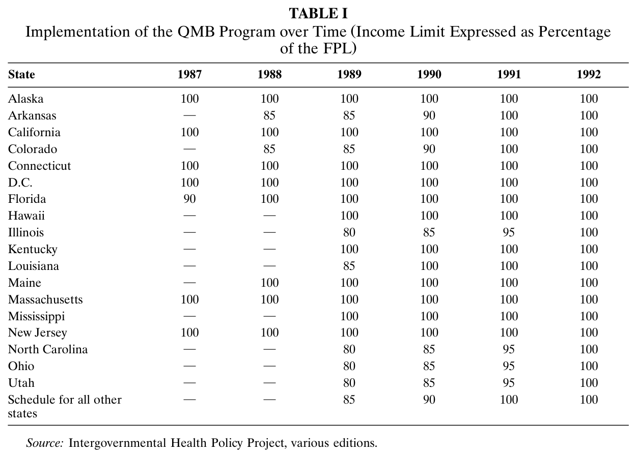
The QMB income limits (expressed as a percentage of the poverty line) from voluntary state adoptions between 1987 and 1992 are documented in Table I. From 1987 to 1990, several states implemented the QMB expansions prior to the federal mandates.
These states typically adopted an income limit of 100% of the poverty line. The states included California, the District of Columbia, Florida, Hawaii, Maine, Massachusetts, Mississippi, New Jersey, New York, Pennsylvania, and South Carolina. These voluntary adoptions create additional variation beyond the federal mandates to identify the effect of the QMB laws on SSI participation.11
This QMB coverage itself represents a valuable benefit to an elderly individual. In 1993, the national average actuarial value of the QMB program was $950 per year, and the minimum benefit was $439 (the annual Medicare Part B premium for a QMB who received no services during the year). Out-of-pocket costs would be reduced by over $2,300 per year for a beneficiary who has a typical hospitalization and skilled nursing facility stay during the year.12
### Table I. Implementation of the QMB Program over Time (Income Limit Expressed as Percentage of the FPL)
Table I. Implementation of the QMB Program over Time (Income Limit Expressed as Percentage of the FPL) — source page 4. Open full-resolution image · Read source PDF page
## III. THEORETICAL CONSIDERATIONS
### Basic Model
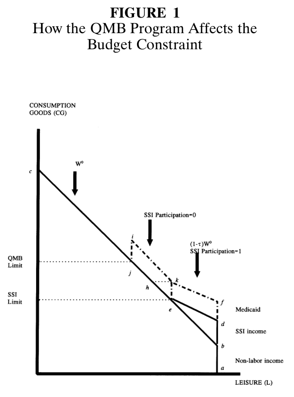
I assume that an elderly individual (or household) maximizes his utility subject to a budget constraint. Utility is assumed to be a function of leisure and consumption goods, , and the price of consumption goods is normalized to $1 per unit. The individual may have some form of nonlabor, nontransfer income (for instance, income through Social Security or private pensions). If the elderly individual chooses to work, he earns a wage, , in the labor market. This results in the budget set in Figure 1.
By introducing the SSI system, the government offers a grant () and reduces it at a tax rate ().13 This results in the budget set given by . After the introduction of SSI, the recipient’s after-tax wage falls from to on the part of the budget segment spanning . The income limit where SSI eligibility ends is a weighted average of the limits given in equations (1) and (2) in section II, depending on the mix of nonlabor, nontransfer income and earnings.
SSI’s treatment of Medicaid benefits is quite different from its treatment of cash benefits. A beneficiary receives Medicaid when participating in SSI and loses it completely when leaving SSI. This creates the budget segment given by . Clearly the loss of Medicaid creates a certain segment of the budget set (segment ) where the individual could receive higher utility by instead locating at point . This discrete loss of health insurance benefits is known as the “Medicaid notch.” The QMB expansions change the budget set further, by allowing a recipient to receive Medicaid without the need to participate in SSI. This now changes the budget set to . Compared to the budget set before the QMB expansions (segment ), this model predicts that SSI participation should fall or remain unchanged if there is no behavioral response. The reasoning behind this prediction is that all the new bundles on segment occur where the individual does not participate in SSI.
An increase in earnings is only one of three reasons why an individual or household would leave SSI. As Moffitt [1983] has noted, welfare can be stigmatizing. The utility function discussed earlier could then be modified to where stands for the disutility of participation in the SSI or QMB programs. If collecting a cash handout is more stigmatizing than collecting Medicaid alone, then an individual who was initially on SSI may decide to leave after the QMB expansions, and thus give up his cash benefits.
### Figure 1. How the QMB Program Affects the Budget Constraint
Figure 1. How the QMB Program Affects the Budget Constraint — source page 5. Open full-resolution image · Read source PDF page
**Caption:** How the QMB Program Affects the Budget Constraint
Finally, the QMB expansions had asset limits that were double those of SSI. Thus, a single individual could have as much as $4,000 of assets under QMB, while a married couple could have $6,000. If a household prefers accumulating higher assets than SSI allows, it might choose to leave SSI and join the QMB program instead. Neumark and Powers [1998] find that higher SSI benefits reduce saving among households with heads who are approaching the SSI eligibility age and are likely participants in the program.
### The Role of Information
The theoretical model assumed perfect awareness about SSI benefits, but this assumption is clearly false.14 If awareness about SSI is a serious problem, then the QMB expansions could increase SSI participation.
Some states took active efforts to inform QMB recipients of their eligibility. These effects included the distribution of press releases, toll-free telephone “hot line” numbers, brochures, fact sheets, and public service announcements.15 Another possibility is that some health shock may land the individual in the hospital, where he learns about the QMB program and other welfare benefits available to him. In either case, he perceives his original budget set (before the QMB expansions) to be rather than , and after the expansions . In this case, the expansions may increase SSI participation: after learning about SSI, he may choose to enroll in SSI and locate somewhere along the segment , or he may choose to not enroll, and locate somewhere along segment .
## IV. DATA DESCRIPTION
### Operationalizing the QMB Expansions
As described in section III, changes in QMB law could increase or decrease SSI participation. The budget constraint in Figure 1 illustrates a way to represent the QMB expansions. Essentially, the QMB expansions amount to changing the income limit for Medicaid, possibly above the SSI income limit. By setting the price of consumption goods at $1 per unit, the y-axis in this figure measures the maximum income limit for Medicaid before and after the QMB expansion. This can be denoted as:
**Equation (3):**
where stands for the annual Medicaid income limit (in dollars) and stands for the annual SSI income limit. therefore represents the increase in the income limit for Medicaid above and beyond the income limit for SSI (in other words, how drastically has the budget constraint for the individual changed). I take the maximum of this number and zero, because there are instances when a QMB expansion (to, say, 85% of the poverty line) is less generous than the SSI income limit. In this case, the Medicaid income limit is not lowered, but remains unchanged.
Measuring QMB is straightforward: the Medicaid income limit is imputed for a person based on his state of residence, time period, and the federal poverty line. The SSI income limit is computed from the state rules, time period, family circumstances, and the individual’s Social Security income. By including as an explanatory variable for SSI participation, the preceding analysis shows we would expect a negative coefficient—intuitively, weakening the link between Medicaid and SSI will reduce SSI participation.
In addition to the variable , I include four other policy variables. The first is the SSI limit itself. Raising the SSI income limit (everything else held constant) should increase SSI participation. The second is a dummy variable for whether the individual’s state had implemented a QMB expansion. If individuals learn about SSI through the QMB program, then the implementation could increase participation. The third is the MN limit. Technically, the QMB program did not “break the link” between SSI and Medicaid, because the MN program is not conditional on SSI participation. It is expected that SSI participation should be lower, when the MN limit is higher. Finally, I include a dummy variable for whether the respondent lived in a 209(b) state—that is, a state where he must file a separate application for Medicaid and possibly face stricter standards for Medicaid eligibility. Because of these hassles, living in a 209(b) state should reduce SSI participation.
### Current Population Survey Data, 1987-1992
I use repeated cross-sections from the March Current Population Survey (CPS). The CPS is a nationally representative data set that surveys approximately 50,000 households. In addition to demographic characteristics, the March Annual Demographic File provides retrospective information on income and health insurance sources such as SSI income, Social Security income, and Medicaid. Therefore the 1988 to 1993 surveys provide information from calendar years 1987 to 1992.
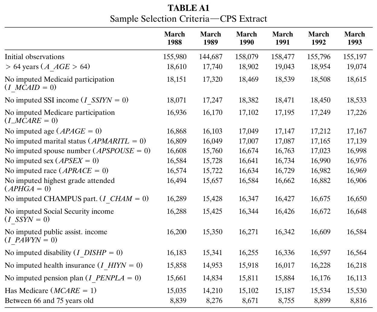
When compared to other data sets, such as the Survey of Income and Program Participation (SIPP), the CPS has some advantages and disadvantages for examining Medicaid’s impact. The CPS is an excellent starting point, because it provides data in a more timely fashion, which facilitates examining recent changes in law. In addition, the CPS uniquely identifies every state and has larger sample sizes than the SIPP. The CPS has some drawbacks, however. The key outcome, SSI participation, is defined as whether the respondent received any SSI income in the previous year. This retrospective information could be subject to recall bias. Also, even if the QMB program removed the elderly from the SSI rolls partway through the year, the respondent would still correctly claim he participated in SSI. Thus, this aggregation likely understates the effectiveness of the QMB laws. In addition, the respondent may not report SSI participation, either because of confusion about the program’s name (such as the distinction between SSI and AFDC) or because of the stigma in admitting welfare participation. Finally, the CPS does not directly report asset holdings, a point I address later. The SSI eligibility rules prohibit individuals with more than $2,000 in assets (and families with more than $3,000) from applying to the program. From the CPS, I extract respondents aged 66 to 75. This encompasses the same age range that Friedberg [1997, 1999] studied when she examined the effects of Social Security and Old Age Assistance on the elderly. Thus, this is an elderly sample where we might expect some changes in labor supply when the budget constraint changes. The labor force participation rate for my CPS sample varied between 15%-16% during the time period. I exclude individuals with imputed information on SSI eligibility. In addition, I exclude elderly respondents who do not report Medicare coverage, since QMB eligibility requires the individual to be eligible for Medicare (this eliminates roughly 5% of the elderly sample). To the remaining observations, I attach information on QMB eligibility derived from Intergovernmental Health Policy Project documentation.
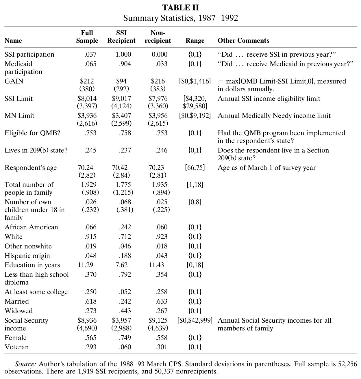
The CPS sample consists of 52,256 observations.16 The means of the variables used in the analysis are shown in Table II. The dependent variable, SSI participation, averages 3.7%. Although not shown, several of the policy variables change quite dramatically over time. The variable GAIN—the increase in the income limit above the SSI limit, averages $212. It increases more than tenfold during the period, from an average of $31 in 1987 (when only a few states had implemented optional mandates) to an average of $455 in 1992 (when binding federal mandates forced all states to cover all senior citizens under the poverty line). The variation in Social Security income (which has a mean of $8,936 and a standard deviation of $4,690) leads to considerable variation in the SSI income eligibility limit, which averages $8,014. The demographic composition of the sample remains fairly stable over time. Family size averages 1.9 people. The average age of the respondent is 70.24 years (this increases slightly, from 70.2 to 70.3 during the period). Approximately 6.6% of the sample are African American and 91.5% are white. Around 4.8% are Hispanic. Nearly 57% are female, and almost 30% are veterans. More than 60% of the sample are currently married, and more than 25% are widowed. Around 37% did not complete high school, while 25% had some college education.
The table also breaks the sample out into SSI recipients and nonrecipients. The two groups differ considerably along many of the demographic dimensions. SSI recipients are more likely to be nonwhite, or of Hispanic origin. They are far less educated, more likely to be single, to be female, and to have lower levels of Social Security income. They tend to live in more generous SSI states, as reflected through the SSI limit.
### Table II. Summary Statistics, 1987-1992
Table II. Summary Statistics, 1987-1992 — source page 8. Open full-resolution image · Read source PDF page
**Notes:** Source: Author’s tabulation of the 1988-93 March CPS. Standard deviations in parentheses. Full sample is 52,256 observations. There are 1,919 SSI recipients, and 50,337 nonrecipients.
## V. RESULTS
This section is divided into five parts. The first part sets up the regression framework and explains how the estimates account for other stories that could potentially contaminate the inferences. It then presents results from the CPS sample, along with cost estimates of the QMB program. The second part illustrates how the QMB effect varies by demographic group. The last three parts check the robustness of the initial findings.
The third part addresses some concerns about asset holdings. The fourth part checks the robustness of the findings to other parameterizations of the policy variables that do not rely on the individual’s Social Security income. The fifth part explores the comparability of the “treatment” and “control” groups.
### Basic Results from the Full CPS Sample
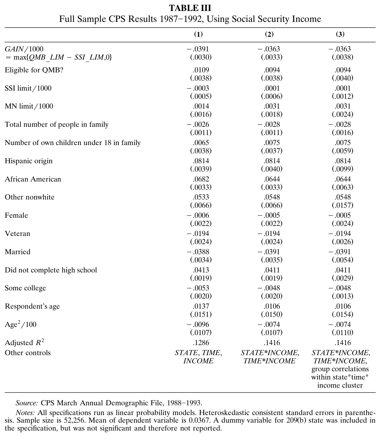
The outcome of interest is whether or not the respondent participated in SSI. For ease of presentation, I show results from a linear probability model. The preferred specification, presented in Table III, column (3), and all the tables that follow, is:17
**Equation (4):**
Here is an indicator variable equal to 1 if individual participated in SSI; represents the dollar difference between the QMB and SSI income-eligibility limits as a function of state, time, and Social Security income; is an indicator variable equal to 1 if individual 's state had implemented a QMB expansion; is the SSI income-eligibility limit in dollars; is the Medically Needy income limit; is an indicator variable equal to 1 if the respondent lives in a Medicaid 209(b) state; and is a vector of other individual characteristics that may affect SSI participation, such as age, gender, ethnicity, and race. is a residence-state dummy, ; is a Social Security-income-category dummy in intervals through , ; and is a calendar-year dummy, . The coefficients , , and are estimated, and is an error term assumed to be uncorrelated with the explanatory variables. The model in section III predicts , , , , and .
By including and , the specification controls for unmodeled state-specific or time-specific factors that may affect SSI participation. If these omitted variables are correlated with and affect SSI participation, then the coefficient will be biased without their inclusion. In 1990, for instance, Congress established federal minimum standards for marketing and selling Medigap policies.18 If this nationally uniform reform in the Medigap insurance market reduced SSI participation because the private health-insurance alternative to Medicaid became more attractive, then the coefficient on may also capture this effect without the time dummies. Inclusion of state dummies could control for variation in access to or quality of health-care facilities.
The SSI income-eligibility limit is calculated based on the generosity of state and federal benefits, household composition, and the individual's or family's nonlabor, nontransfer income through Social Security. This study exploits this additional variation in the limit due to nonlabor income because SSI law requires that SSI applicants file for all other benefits for which they are entitled. Since its inception SSI has been viewed as the “program of last resort.” That is, after evaluating all other income, SSI pays what is necessary to bring an individual to the statutorily prescribed income floor.19
As of September 1992, 68% of aged SSI recipients also received Social Security. Social Security benefits are the single highest source of income for SSI recipients.20 The more income the family receives through Social Security, the lower the SSI income limit, with the limiting case being the SSI income limit calculated in equation (1) in section II. Although other sources of nonlabor income, such as pension income, dividends, and interest, could be included, I prefer to exclude these more portable sources that could be transferred to the respondent's children if the parent anticipated participating in SSI.21
### Table III. Full Sample CPS Results, 1987-1992, Using Social Security Income
Table III. Full Sample CPS Results, 1987-1992, Using Social Security Income — source page 10. Open full-resolution image · Read source PDF page
I was also concerned that Social Security income itself may be correlated with SSI participation in ways other than its direct effect on the SSI income eligibility limit and GAIN. For instance, if respondents with higher Social Security income have more attachment to the labor force, a larger stigma cost of participating in SSI, or higher savings, then the estimate on the SSI income limit and GAIN may not represent variation in program rules, but rather different preferences. To control for this possibility, I included a set of dummy variables for different levels of Social Security income. Moreover, I added interactions of these six income dummies with the fifty state dummies, and also with the five time dummies.
These interactions may help control for the possibility that states have other transfer programs for the poor elderly or have different amounts of bureaucracy in applying for SSI. Similarly, if other programs (such as General Assistance) were being scaled back in all states over time, its effect on SSI participation would come through the interaction of and . I will explore this point later, by using other measures of the SSI limit that do not rely on the individual's measure of Social Security income.
The findings on SSI participation for the full sample are presented in Table III.22 As we move across the three columns, the model adds a more detailed set of dummy variables.
In all specifications, increasing the Medicaid income limit significantly reduces SSI participation. The most careful specification, column (3), corresponds to the model in equation (4). The coefficient estimate on GAIN reads: increasing the income limit for Medicaid by $1,000 beyond the SSI limit would result in a reduction in SSI participation of 3.6 percentage points. In the absence of the QMB expansions this model implies that SSI participation would have been 1.7 percentage points higher, or 45% higher than it actually was, because the fully phased-in QMB expansions increased GAIN by roughly $455 in 1992. In terms of number of people leaving SSI, this corresponds to 240,000 respondents in the CPS sample. Since administrative numbers from HCFA show that 885,000 senior citizens were covered by QMB in calendar year 1992, and approximately 42% of elderly Medicaid eligibles were between 66 and 75, then more than 60% of those covered were previously insured by Medicaid through SSI.23
It is not possible to directly compare my number to other estimates, because no previous study has estimated the impact of Medicaid on SSI participation.24 Similar estimates exist in AFDC literature, however. In previous work, I found that increasing the Medicaid income limit above the AFDC income limit by $1,000, for a family of three, results in a 1.8 percentage point drop in AFDC participation (Yelowitz [1995]). Thus, it appears that Medicaid is more important in the SSI participation decision of the elderly than in the AFDC participation of female heads.
Does this help us understand how expensive the QMB program really was? In 1992, the average payment to an aged individual was $196 per month, and to an aged couple $414 per month. Thus the average aged recipient received around $2,400 in SSI benefits during that year. The results from above imply that, for the elderly aged 66 to 75, the SSI caseload would have been 240,000 higher than the 663,000 actual SSI recipients if the QMB buy-in program did not exist.25 This implies a saving to the SSI program of $576 million. On the other hand, around 1.4 million QMB beneficiaries had joined by the end of 1992 (General Accounting Office [1994]), of which approximately 42% fell into this age range. If these beneficiaries valued the buy-in coverage at its actuarial value (roughly $950 per year), then this implies a cost of $559 million. Thus, the QMB program was considerably less expensive than one would calculate from simply examining the increased health care expenditure, and may have even been self-financing through reductions in SSI participation.
The second policy variable asks whether the respondent’s state had enacted any form of the QMB buy-in program. From 1989 onward, every state was forced by federal mandate to implement the program, but there is variation across states in 1987 and 1988. If learning about the SSI program is facilitated through the existence of the QMB program, then the sign on this variable should be positive. The existence of the QMB program is associated with an increase in SSI participation of 0.9 percentage points, as shown in Table III, column (3). This significant positive association also appears in most of the alternative specifications in the subsequent sections.
The results on increasing the SSI limit are weaker than those on increasing the Medicaid limit. Increasing the SSI limit by $1,000 is associated with an increase in SSI participation of 0.1 percentage points, and is insignificant for the full sample. Moreover, the economic magnitude is much smaller than the effect of increasing the limit in the first row. The coefficient also varies in sign and statistical significance in the models that follow. The coefficient is correctly signed for demographic groups that are more disadvantaged, but usually imprecisely estimated for other groups.
The findings on the demographic variables in the first column are expected. African Americans, other nonwhites, and those of Hispanic origin have significantly higher propensities to participate in SSI.
These groups are more likely to be familiar with other welfare programs such as AFDC, and live in urban areas with greater access to welfare offices. Being female increases participation, while being a veteran lowers participation by 1.9 percentage points. This is reasonable since veterans may have pension income or alternative sources of health insurance coverage from the military. Those with less than a high school diploma are significantly more likely to participate in SSI.
Again, this could reflect a history of welfare participation, lower stigma costs, superior information about SSI, lower income, or lack of pension coverage. Relative to respondents who completed high school, being in the dropout group raises the participation probability by 4.1 percentage points. Respondents who completed at least some college are less likely to participate compared to those who completed only high school, but the difference in participation rates is not as dramatic.
### Demographic Differentials in the Effect of QMB
Several studies find different responses to welfare policy across demographic groups.
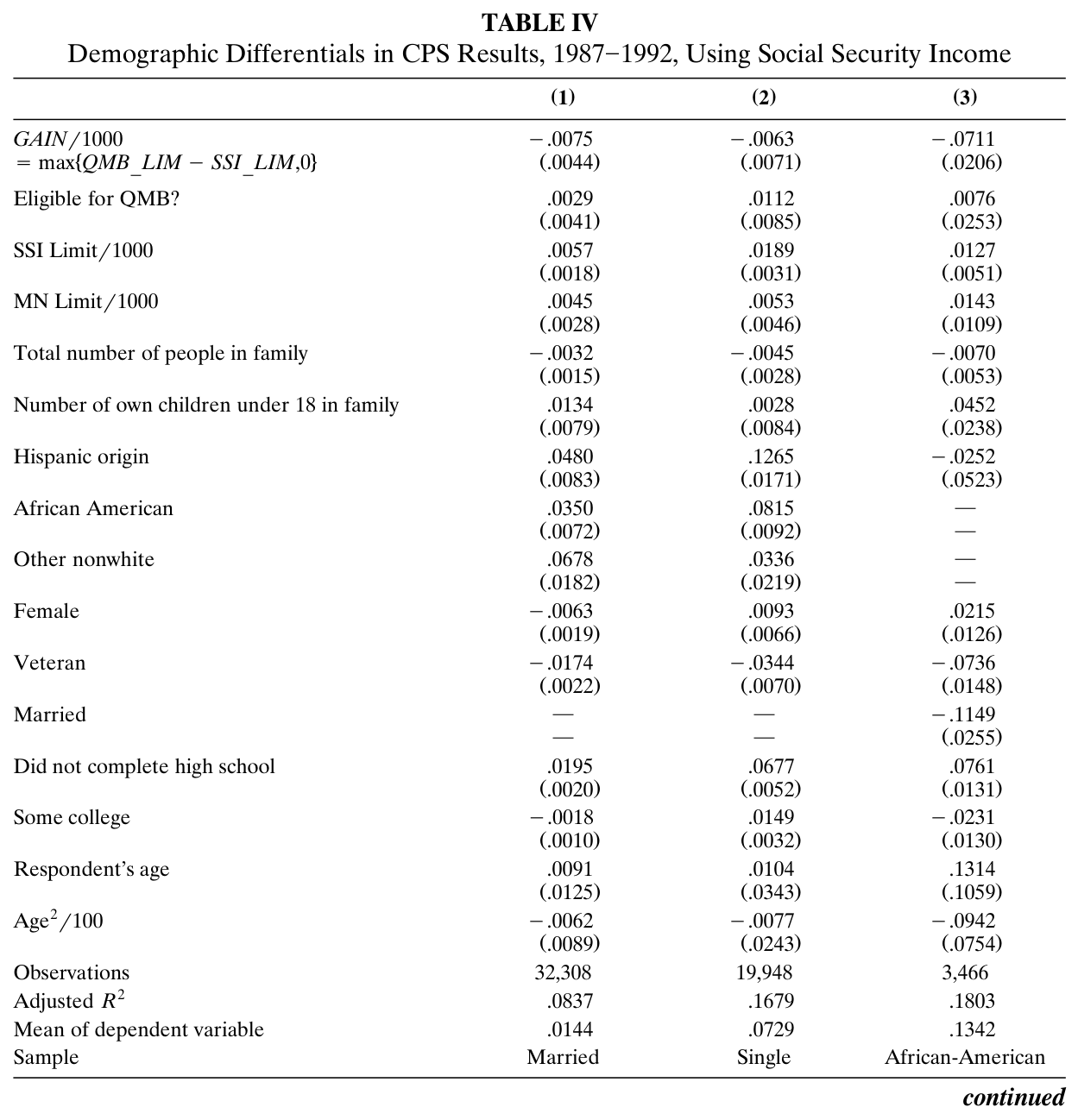
To analyze the ultimate incidence of the QMB reforms, it is important to see whether all groups benefited equally by the QMB coverage. Table IV, columns (1) and (2), divides the sample into married and single individuals.
For both groups the QMB expansions reduce SSI participation, though the effect is smaller for single respondents (and not significant). The coefficients on several explanatory variables change signs and the coefficient estimates on others change magnitude, which suggests an interaction effect between them and marital status. Most notably, the SSI limit has a much bigger positive effect on single individuals, an effect that is larger than from increasing the QMB limit by the same dollar amount. Being a single woman raises the probability of SSI participation, while being a married woman lowers it. While it may seem puzzling that being female lowers SSI participation, recall that both Social Security income and marital status are controlled for.
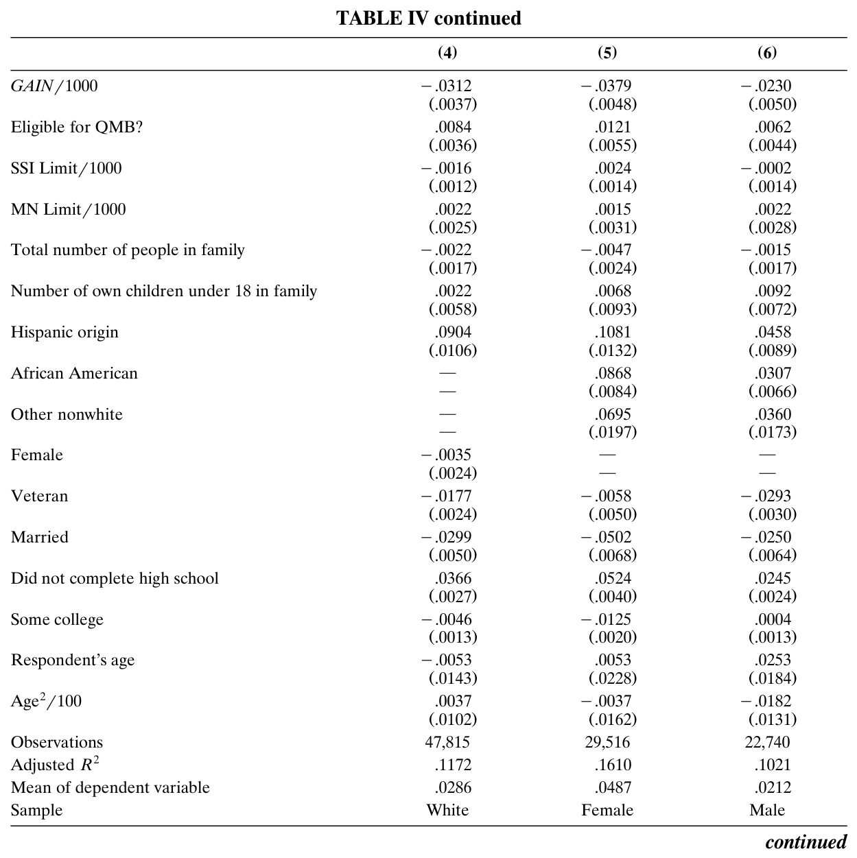
Does the effect vary by race? I examine this in columns (3) and (4) by dividing the sample into African Americans and whites (I exclude the other nonwhite category from the analysis). While increasing the income limit results in significant reductions in SSI participation for both groups, the estimated effect is much stronger for African Americans, and we can reject that the coefficients are equal. Increasing the income limit by $445 reduces SSI participation by more than 3.2 percentage points for African Americans. The African American caseload would have been almost 25% higher in 1992 without the buy-in program. This strong result might be attributable to the likelihood that many African Americans do not have retiree health insurance from a previous employer, and so are more dependent on SSI to provide a health insurance policy. A policy change that offered health insurance coverage off of SSI would therefore have stronger effects. Chulis, Eppic, Hogan, Waldor, and Arnett [1993] find that only 20.2% of elderly African Americans had employer-sponsored retiree health insurance, compared with 34.6% of whites. Another explanation is that African Americans are better informed about the availability of welfare benefits, which implies that the introduction of the QMB program would be less likely to increase SSI participation. This may explain the insignificant coefficient on QMB eligibility in column (3).
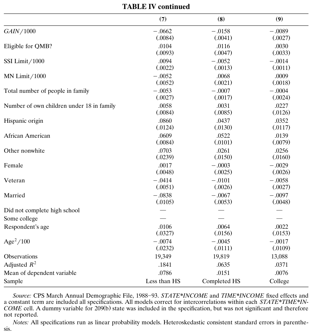
Columns (5) and (6) examine gender differences. The expansions appear to have a greater effect on reducing SSI participation for women than men, though the caseload reductions from a $1,000 change in the income limit are similar. Again, this may be due to the availability of retiree health insurance. Chulis et al. (1993) also find gender differences in private health insurance coverage. Approximately 38% of men had retiree health insurance through their employer, compared to 30% of women. Finally, education differences are examined in columns (7), (8), and (9). These columns show, successively, that the buy-in program had larger effects on the less educated. Increasing GAIN by $1,000 leads to a fall in SSI participation of 6.6 percentage points for high school dropouts, whereas the same policy change leads to a fall of just 0.9 percentage points for college-educated respondents.
### Table IV. Demographic Differentials in CPS Results, 1987-1992, Using Social Security Income
Table IV. Demographic Differentials in CPS Results, 1987-1992, Using Social Security Income — source page 13, part 1 of 3. Open full-resolution image · Read source PDF pageTable IV. Demographic Differentials in CPS Results, 1987-1992, Using Social Security Income — source page 14, part 2 of 3. Open full-resolution image · Read source PDF pageTable IV. Demographic Differentials in CPS Results, 1987-1992, Using Social Security Income — source page 15, part 3 of 3. Open full-resolution image · Read source PDF page
### Accounting for Asset Holdings
The preceding estimates have ignored the fact that an individual must also have low asset levels to qualify for SSI. Unlike other segments of the population, many senior citizens do indeed have assets. The liquid asset limit is currently $2,000 for individuals and $3,000 for married couples. The asset limits changed modestly during the period I studied, but were always very low.
The Social Security Administration (SSA) is quite vigorous in enforcing the asset rules. It receives information from the Internal Revenue Service on an applicant’s nonwage income, mainly interest payments submitted to the IRS by financial institutions, dividend income, and unemployment compensation. SSA currently examines cases where this reported income exceeds the limit by as little as $41.
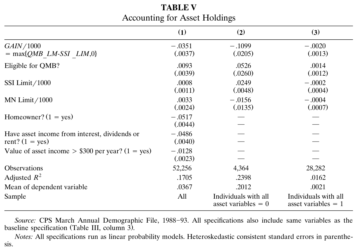
Unfortunately, the CPS only has crude measures of assets. I amend the model to include three measures. I include a dummy variable for whether the respondent owned his home. Although the SSI rules do not count a home in determining eligibility, owning a home is correlated with other forms of wealth. I also include a dummy variable for whether the respondent’s family had any income in the form of interest, dividends, or rent. Finally, I add a dummy variable for whether the sum of these three income sources was greater than $300 per year. Assuming that the rate of return on these assets is 10%, this sum would correspond to having asset holdings in excess of $3,000—making the respondent categorically ineligible for SSI.26
The results are shown in Table V. Column (1) includes these variables in the regression directly, and it includes the other covariates in the baseline specification. Compared to the model that omitted these asset variables, the coefficient estimate barely changes. The adjusted R* increases, however. In addition, all three asset variables have significant negative effects on SSI participation. The second column examines 4,364 individuals who have all three of these asset variables set equal to zero. For this group, the effect of GAIN is much stronger than for the whole sample, as expected. The final column examines 28,282 individuals with all the asset variables set equal to one. The effect of the QMB reforms on this group is around 50 times smaller than the effect is on those without any assets.
### Parameterizations of the Policy Variables Not Using An Individual’s Social Security Income
All of the prior estimates rest on the assumption that Social Security income is exogenous. While this may be reasonable, there are two key arguments on why Social Security’s influence may not come through the policy variable GAIN (as well as the SSI limit). First, preferences vary across individuals. If a person has a strong labor force attachment during his life and a high stigma cost to welfare participation, then he is likely to have high Social Security benefits.27 This translates into a lower SSI limit and a higher value of GAIN. Since this person also has a lower propensity to participate in SSI, then the larger value of GAIN associated with this person could lead to a spurious finding that the QMB laws reduce SSI participation.
### Table V. Accounting for Asset Holdings
Table V. Accounting for Asset Holdings — source page 16. Open full-resolution image · Read source PDF page
**Notes:** Source: CPS March Annual Demographic File, 1988-93. All specifications also include same variables as the
**Notes:** Notes: All specifications run as linear probability models. Heteroskedastic consistent standard errors in parenthe-
If the model were only estimated within a single state at a point in time, then the variation in GAIN would reflect preferences rather than the budget constraint—which means that we do not learn about the QMB laws. By and large, this is addressed through the comparisons across states and over time within a given income group. By including INCOME controls (or interactions of STATE*INCOME and TIME\*INCOME), the variation in the GAIN variable comes from changes in the QMB laws within a given income group.28 Conceptually, the regression compares groups of individuals with similar Social Security levels who live in different states, or similar income groups in different time periods who face different Medicaid regimes.
A second criticism of using Social Security income is that it may be endogenous to the SSI program rules. To understand why, we need to understand how Social Security benefits are determined. The benefits are computed based on average indexed monthly earnings (AIME), the age at which benefits are drawn, the recipient’s family status, and current earnings levels for those between the ages of 62 and 69. While a person approaching the age of 65 who is contemplating SSI participation may not be able to substantially influence the AIME level (since it is determined from the recipient’s 40 years of highest earnings), he has some choice over his retirement age. If he retires at age 62, he gets just 80% of the Social Security benefit he would receive at 65. If he delays retirement past 65, the benefits increase by 3% per year (until age 72). Moreover, his work (and hence, welfare) decisions between ages 62 and 69 influence his Social Security benefit through the retirement earnings test.
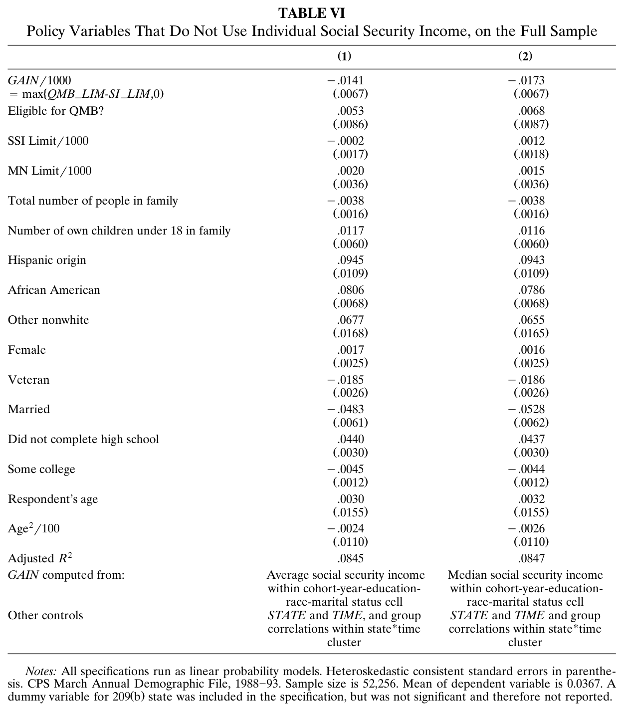
Because of both concerns, it is important to try measures of GAIN (and the SST limit) that do not rely on the individual’s own Social Security income. I reestimated the model including measures of Social Security income constructed from the mean (and also, median) Social Security values within a birth cohort/marital status /education/race /year cell.29 In this way, the construction of GAIN is not as susceptible to the criticism that it is influenced by an individual’s decisions. The method does have a tradeoff, however, in that it adds a great deal of measurement error to the policy variables. The results are presented in Table VI.30 In both columns, raising the Medicaid limit still reduces SSI participation. The coefficient estimate on GAIN is less than one half of the size in the baseline specification, however. To some extent, this is expected, because of the measurement error in GAIN.
### How Comparable Are the “Treatment” and “Control” Groups?
The whole motivation for using some source of nonlabor income to construct GAIN is that many elderly are not going to be on the margin of SSI participation. This section explores whether the prior findings are very sensitive to changes in the sample selection, and to constructing GAIN using finer intervals of Social Security income.
I modify the baseline specification by restricting the sample to elderly individuals who report Social Security income of less than $7,500. By doing so, the aim is to restrict the sample to individuals who are “at risk” of participating in SSI. In addition, the previous income categories were somewhat large—there could be a fair degree of heterogeneity even within the INCOME cell. A person with $4,999 in Social Security income may not be comparable to a person with $1, but the previous specifications would classify them in the same group.
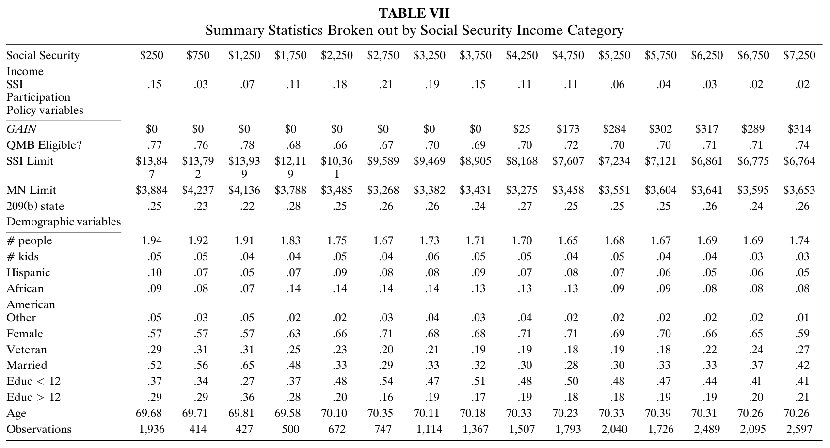
From this smaller sample of 21,424, I classify individuals into fifteen income intervals ranging from $0—$500, $500-$1,000,..., up to $7,000—$7,500. For each individual in that interval, I assign the midpoint of the Social Security value to construct GAIN (i.e., $250 for the first category, and $7,250 for the last).
Therefore, all individuals within an income group, in one state at a single point in time, will have the SSI limit. The means of observable variables for each group are shown in Table VII. Casual inspection shows that the demographic variables stay fairly steady across income groups.
There appear to be differences in observable characteristics between those with very low levels of Social Security income (ie., $250-$1,750) and those with somewhat higher levels (i.e., over $3,000), however. In particular, the number of people in a household drops for the higher income groups, while the percentage who are female or single increases. SSI participation declines for higher income categories, starting at $2,750.
### Table VI. Policy Variables That Do Not Use Individual Social Security Income, on the Full Sample
Table VI. Policy Variables That Do Not Use Individual Social Security Income, on the Full Sample — source page 18. Open full-resolution image · Read source PDF page
**Notes:** Notes: All specifications run as linear probability models. Heteroskedastic consistent standard errors in parenthesis. CPS March Annual Demographic File, 1988-93. Sample size is 52,256. Mean of dependent variable is 0.0367. A dummy variable for 209(b) state was included in the specification, but was not significant and therefore not reported.
For lower income categories, however, the pattern is not as clear. In particular, the first income category has a much higher participation rate than the other categories close to it. Finally, the Medicaid policy was not binding for income groups below $4,250.
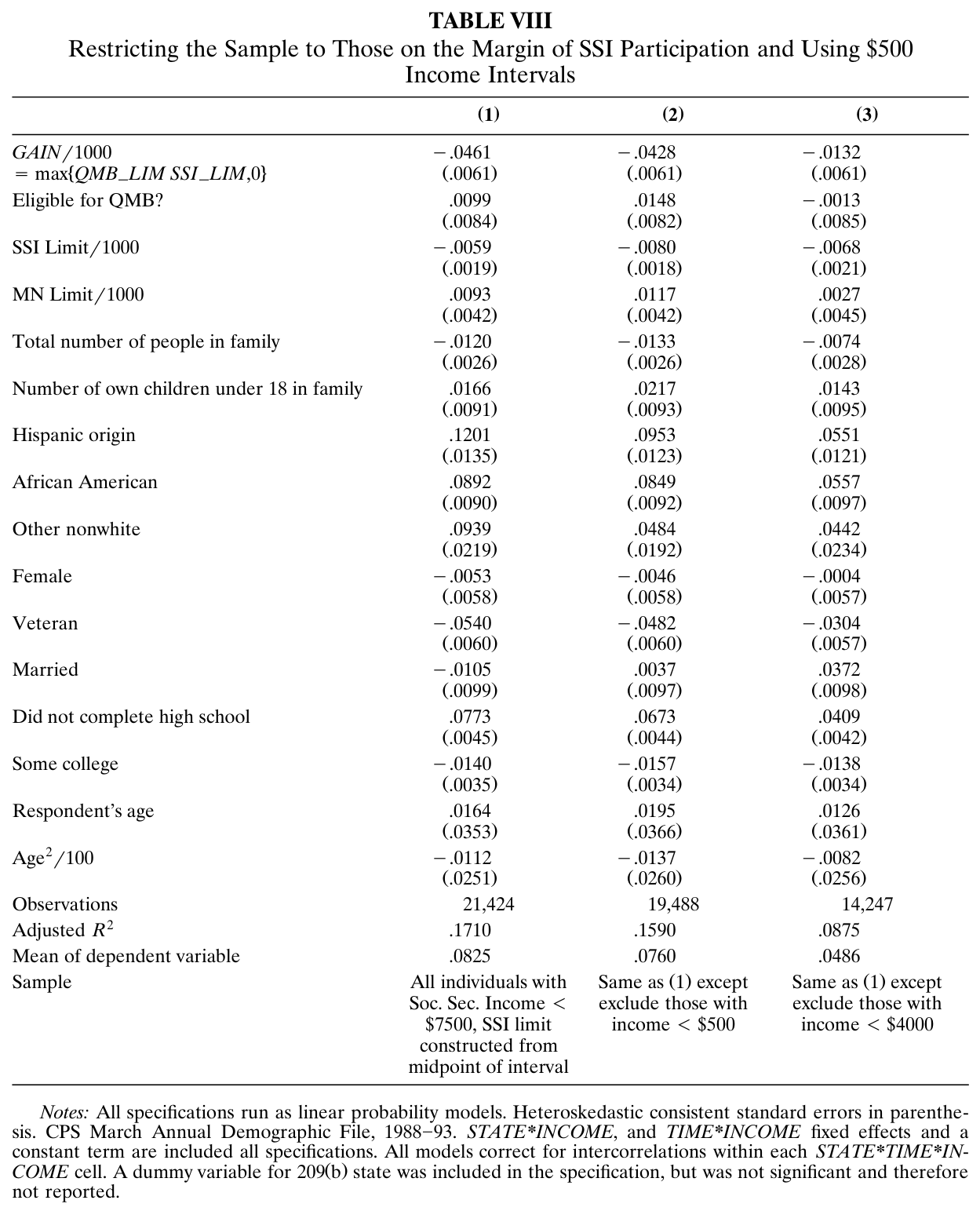
Table VIII presents three additional specifications, motivated by the patterns in the previous table. The first column shows the results for all individuals with income less than $7,500. The model includes interactions of the fifteen income categories with the state dummies, as well as with the time dummies. The second column excludes those in the lowest income group of $0 to $500, since Table VII shows some differences between this group and the others. The third column includes those with incomes between $4,000 and $7,500, since the QMB expansions only change the budget constraint for this part of the sample.
The first two columns present very similar findings on QMB policy. In both cases, increasing the QMB limit reduces SSI participation. The final column, which only examines groups where GAIN was positive, shows smaller findings than the first two columns. In addition the SSI income limit variable is incorrectly signed.
### Table VII. Summary Statistics Broken out by Social Security Income Category
Table VII. Summary Statistics Broken out by Social Security Income Category — source page 19. Open full-resolution image · Read source PDF page
### Table VIII. Restricting the Sample to Those on the Margin of SSI Participation and Using $500 Income Intervals
Table VIII. Restricting the Sample to Those on the Margin of SSI Participation and Using $500 Income Intervals — source page 20. Open full-resolution image · Read source PDF page
**Notes:** Notes: All specifications run as linear probability models. Heteroskedastic consistent standard errors in parenthesis. CPS March Annual Demographic File, 1988-93. STATE*INCOME, and TIME\*INCOME fixed effects and a constant term are included all specifications. All models correct for intercorrelations within each STATE\*TIME\*INCOME cell. A dummy variable for 209(b) state was included in the specification, but was not significant and therefore
Overall, three conclusions can be made from this section. First, at least on observable characteristics, there are not dramatic differences between the income categories. Second, by looking at those who are on the margin for SSI eligibility, the impact of the QMB law increases compared to the full sample. Third, the findings on the SSI limit are more sensitive in this framework. Dropping the lowest income category affects the results on the SSI income limit.
## VI. CONCLUDING REMARKS
Although the majority of policy attention devoted to the QMB program has focused on the pattern of less-than-full take-up, the program appears to have the important consequence of reducing SSI participation. This article has shown sizable effects on SSI participation of decoupling health insurance coverage from SSI eligibility. The QMB expansions show the most dramatic effects for African Americans and the least educated.
Cost estimates show that the program may come close to paying for itself. During the 1980s and 1990s, the caseload growth of disabled SSI beneficiaries shot up dramatically, while the caseload growth of elderly SSI beneficiaries was minimal. Why then do I focus my analysis on the elderly population? The first reason is practicality.
The definition of the elderly group remained constant during the sample period and this group is clearly identifiable in the CPS data. In contrast, only self-reported, rather than objective, measures of disability are available in the CPS data. In addition, disability reporting may be a function of the generosity of the SSI program.31 Also, there were some changes in evaluating disability over the sample period. For instance, the Supreme Court’s 1990 Sullivan v. Zebley decision resulted in a revised definition of disability for children under the age of 18. The second reason is policy-oriented. If we can explain why the elderly caseload remained stable, while the caseloads of other entitlement programs such as AFDC, Food Stamps, and Medicaid increased dramatically, then we may be able to offer policy proposals that will control the caseload growth in other programs.
Recent proposals for Medicaid reform would cut back on the QMB expansions for elderly (and perhaps also the Medicaid coverage of pregnant women and children). This study helps illustrate the full consequences of such on costs, by emphasizing the link to SSI. By scaling back eligibility, the states may assist senior citizens in moving onto the federal SSI rolls.
The analysis will be extended in three directions. First, this article has focused on the effects of delinking the Medicaid and SSI program. It has not focused on the role of health in determining SSI participation. A more complete model of SSI participation that accounted for the effects of health, along the lines of Wolfe and Hill [1995], could help determine what type of person was likely to leave SSI from the QMB program. Second, it is important to know the extent to which the QMB program crowded out private Medigap purchases. Cutler and Gruber [1996] find that a significant fraction of newly covered Medicaid beneficiaries among pregnant women and children formerly had some sort of private coverage. To the extent that the QMB coverage simply displaces private coverage, it does not reduce the number of uninsured. A similar crowd-out effect for the elderly may occur in the Medigap market.
Finally, since it appears that Medicaid is an important determinant of SSI participation for the elderly, is the same true for the disabled population? Could offering health insurance off of SSI slow the caseload growth in the SSI disabled program? In other work, I use the variation in Medicaid expenditure across states and over time as a proxy for its value, to assess Medicaid’s importance on SSI participation (Yelowitz [1998a]). In that work, I also find that Medicaid significantly influences SSI participation.
### Appendix Table A1. Sample Selection Criteria—CPS Extract
Appendix Table A1. Sample Selection Criteria—CPS Extract — source page 22. Open full-resolution image · Read source PDF page
## References
Chulis, George, Franklin Eppic, Mary Hogan, Daniel Waldo, and Ross Arnett. “Health Insurance and the Elderly: Data From MCBS.” Health Care Financing Review, Spring 1993, 163-81.
Coe, Richard. “Nonparticipation in the SSI Program by the Eligible Elderly.” Southern Economic Journal, January 1985, 891-97.
Currie, Janet, and Jonathan Gruber. “Health Insurance Eligibility, Utilization of Medical Care, and Child Health.” Quarterly Journal of Economics, May 1996a, 431-66.
———. “Saving Babies: The Efficacy and Cost of Recent Expansions of Medicaid Eligibility for Pregnant Women.” Journal of Political Economy, December 1996b, 1263-96.
Cutler, David. “The Economics of Health and Health Care.” American Economic Review, May 1995, 32-7.
Cutler, David, and Jonathan Gruber. “Does Public Insurance Crowd Out Private Insurance?” Quarterly Journal of Economics, May 1996, 391-430.
Cutler, David, and Brigitte Madrian. “Labor Market Responses to Rising Health Insurance Costs: Evidence on Hours Worked.” Rand Journal of Economics, Autumn 1998, 509-30.
Eissa, Nada. “Taxation and Labor Supply of Married Women: The Tax Reform Act of 1986 as a Natural Experiment.” National Bureau of Economic Research Working Paper No. 5023, 1995.
Friedberg, Leora. “The Labor Supply Effects of the Social Security Earnings Test.” U.C. San Diego Working Paper No. 97-01, 1997.
———. “The Effect of Old Age Assistance on Retirement.” Journal of Public Economics, February 1999, 213-32.
General Accounting Office. “Medigap Insurance: Better Consumer Protection Should Result from 1990 Changes to Baucus Amendment.” GAO/ HRD-91-49, March 1991.
———. “Medicare and Medicaid: Many Eligible People Not Enrolled in Qualified Medicare Beneficiary Program.” GAO/HEHS-94-52, Report, 20 January, 1994.
Gruber, Jonathan, and Brigitte Madrian. ‘‘Health Insurance and Job Mobility: The Effects of Public Policy on Job-Lock.’’ Industrial and Labor Relations Review, October 1994, 86–102.
———. ‘‘Health Insurance Availability and the Retirement Decision.’’ American Economic Review, September 1995, 938–48.
Gruber, Jonathan, and Aaron Yelowitz. ‘‘Public Health Insurance and Private Savings.’’ National Bureau of Economic Research Working Paper No. 6041, 1997; forthcoming Journal of Political Economy.
Hill, Daniel. ‘‘An Endogenously-Switching Ordered-Response Model of Information, Eligibility and Participation in SSI.’’ Review of Economics and Statistics, May 1990, 368–71.
Holtz-Eakin, Douglas. ‘‘Health Insurance Provision and Labor Market Efficiency in the United States and Germany,’’ In Social Protection versus Economic Flexibility: Is There a Trade-off ?, edited by R. Blank. Chicago: University of Chicago Press, 1994, 157–87.
Hubbard, R. Glenn, Jonathan Skinner, and Stephen Zeldes. ‘‘Precautionary Saving and Social Insurance.’’ Journal of Political Economy , April 1995, 360–99.
Intergovernmental Health Policy Project. Major Changes in State Medicaid and Indigent Care Programs, edited by Debra J. Lipson, Rhona S. Fisher, and Constance Thomas. The George Washington University, various editions.
Madrian, Brigitte. ‘‘Health Insurance and Labor Mobility: Is There Evidence of Job Lock?’’ Quarterly Journal of Economics, February 1994, 27–54.
McGarry, Kathleen. ‘‘Factors Determining Participation of the Elderly in SSI.’’ Journal of Human Resources, Spring 1996, 331–58.
McGarry, Kathleen, and Robert F. Schoeni. ‘‘Transfer Behavior in the Health and Retirement Study: Measurement and the Redistribution of Resources Within the Family.’’ Journal of Human Resources , Supplement 1995, S184–S226.
Moffitt, Robert. ‘‘An Economic Model of Welfare Stigma.’’ American Economic Review, December 1983, 1023–35.
Moulton, Brent. ‘‘Random Group Effects and the Precision of Regression Estimates.’’ Journal of Econometrics, August 1986, 385–97.
Neumark, David, and Elizabeth Powers. ‘‘The Effect of Means-Tested Income Support for the Elderly on Pre-Retirement Saving: Evidence from the SSI Program in the US.’’ Journal of Public Economics , May 1998, 181–206.
Poterba, James, Steven Venti, and David Wise. ‘‘Do 401(k) Contributions Crowd Out Other Personal Saving?’’ Journal of Public Economics , September 1995, 1–32.
U.S. Department of Health and Human Services. Medicaid Statistics: Program and Financial Statistics Fiscal Year 1993 . HCFA Pub. No. 10129, October 1994.
U.S. House of Representatives. Medicaid Source Book : Background Data and Analysis . Washington: Government Printing Office, November 1988.
———. ‘‘Outreach Efforts in the Supplemental Security Income and Qualified Medicare Beneficiary Programs.’’ Hearing before the subcommittee on Social Security and the Subcommittee on Human Resources of the Committee on Ways and Means. March 26, 1992.
———. Overview of Entitlement Programs : Background Material and Data on Programs within the Jurisdiction of the Committee on Ways and Means . Washington: Government Printing Office, Various editions.
Wolfe, Barbara, and Steven Hill. ‘‘The Effect of Health on the Work Effort of Single Mothers.’’ Journal of Human Resources, Winter 1995, 42–62.
Yelowitz, Aaron. ‘‘The Medicaid Notch, Labor Supply and Welfare Participation: Evidence from Eligibility Expansions.’’ Quarterly Journal of Economics , November 1995, 909–39.
———. ‘‘Why Did the SSI-Disabled Program Grow So Much? Disentangling the Effect of Medicaid.’’ Journal of Health Economics , June 1998a, 319–49.
———. ‘‘Will Extending Medicaid to Two-Parent Families Encourage Marriage?’’ Journal of Human Resources, Fall 1998b, 833–65.
## Additional printed notes
**1.** U.S. House of Representatives, Overview of Entitlement Programs (1994).
**2.** U.S. Department of Health and Human Services, “Medicaid Statistics: Program and Financial Statistics Fiscal Year 1993.”
**3.** For instance, see Madrian [1994], Holtz-Eakin [1994], and Gruber and Madrian [1994] for evidence on job mobility, Gruber and Madrian [1995] for evidence on early-retirement, and Cutler and Madrian [1998] for evidence on hours of work. Cutler [1995] provides a nice summary of these studies.
**4.** See, for example, Currie and Gruber (1996a, 1996b) for effects on child health, Cutler and Gruber (1996) for crowd-out effects on private health insurance, Gruber and Yelowitz (1997) for effects on savings and consumption, Yelowitz (1995) for effects on labor supply and AFDC participation, and Yelowitz (1998b) for effects on marriage.
**5.** Throughout the article I use the terms “QMB coverage” and “Medicaid coverage” interchangeably, because they offer similar services in terms of Medicare cost sharing.
**6.** I will argue that one of three mechanisms for Medicaid’s effect on SSI participation is through distortions in earnings. Two recent studies show that the labor supply of senior citizens does respond to the parameters of the tax and welfare system in other contexts. Friedberg [1997] shows that the earnings of seniors are reduced by the Social Security retirement earnings test, which often imposes tax rates in excess of 50 percent. Friedberg [1999] shows that the introduction of the Old Age Assistance program (the precursor to SSI) substantially increased retirements in the 1940s and 1950s.
**7.** In reality, SSI eligibility is actually determined on a monthly basis. To keep the analysis consistent with what follows, I convert all numbers from a monthly to an annual basis. There are also asset requirements (known as “resource tests”). A single or widowed recipient may not have more than $2,000 in liquid assets and a married recipient may not have more than $3,000. The value of the recipient’s home is not included, however.
**8.** In the analysis that follows, I compute an individual’s SSI limit by first taking his Social Security income level as nonlabor income, and then assuming the remainder of his income can potentially be in the form of wages.
**9.** These states are known as Section 1634 states.
**10.** In July 1987, for instance, the Medically Needy level exceeded the SSI level in only two states, and these differences were smaller than $10 per month (U.S. House of Representatives, [1988]).
**11.** As with any empirical study that relies on variation in program rules across states, the issue of legislative endogeneity arises. In particular, the states that implemented the QMB program prior to the federal mandates may have done so to reduce the SSI rolls. While it is difficult to think of compelling instruments for early QMB implementation, there are five reasons to believe that this potential problem may be small. First, states were allowed to implement QMB expansions for the elderly only if they also implemented Medicaid expansions for pregnant women and children. This means the cost of getting the elderly off SSI is greatly increased. Second, SSI is mainly financed by the federal government, meaning that the state's incentive to move recipients off the program is reduced. Third, the subsequent empirical results are not sensitive to restricting the sample to states brought into compliance by the federal mandates. Fourth, Section III shows that the theoretical impact of the QMB expansions is ambiguous. Thus, states may not have had enough information to assess whether the QMB expansions would remove senior citizens from SSI. Fifth, the link between QMB and SSI participation is never mentioned in congressional hearings on the QMB program (U.S. House of Representatives [1992]).
**12.** General Accounting Office [1994].
**13.** For simplicity, the figure does not include the standard deduction or work expenses discussed in the prior section, but the predictions will continue to hold by adding in this detail. In addition, Figure 1 also assumes that the value of the QMB program is equal to the value of Medicaid when on SSI. Again, the predictions will continue to hold by making more realistic assumptions.
**14.** The role of program awareness and outreach efforts is discussed in Coe [1985] and Hill [1990].
**15.** General Accounting Office [1994].
**16.** See Appendix Table I for the sample selection criteria.
**17.** The results are qualitatively similar from a logit or probit model. The standard errors on the linear probability model are corrected for heteroskedasticity. In addition, all models control for group correlations within state-year-income cells. Moulton [1986] explains that the standard errors can be understated without correcting for these correlations.
**18.** General Accounting Office [1991].
**19.** U.S. House of Representatives, Overview of Entitlement Programs [1993].
**20.** U.S. House of Representatives, Overview of Entitlement Programs [1993].
**21.** See McGarry and Schoeni [1995] for evidence on transfer behavior from elderly parents to their children.
**22.** In alternative specifications, I have included a state-specific time trend to control for omitted factors within a state that vary over time (such as changing economic conditions) that may be correlated with GAIN and affect SSI participation. The conclusions from these specifications are similar to the ones presented. I have also calculated the SSI limit using all nonlabor, nontransfer income instead of just Social Security income. In these specifications, I again arrive at similar conclusions about the efficacy of the QMB laws.
**23.** This number is computed by taking a weighted average of the number of QMB participants in FY 1992 (which runs from October 1991 to September 1992) and the number of participants in FY 1993. Since 840,000 were covered in FY 1992, and 1,022,000 were covered in FY 1993, this weighted average is 0.75*840,000 + 0.25*1,022,000 = 885,000 participants.
**24.** To the best of my knowledge, just one other study tries to model any aspect of the Medicaid program in the elderly’s SSI participation decision. McGarry [1996] tests whether automatic entitlement to Medicaid, that is not living in a 209(b) state, affects SSI participation. Her findings on the 209(b) are similar to the findings in my study.
**25.** Approximately 45% of elderly SSI recipients are between the ages of 66 and 75. U.S. House of Representatives, Overview Entitlement Programs [1994].
**26.** It is not clear that including these asset variables as exogenous is entirely appropriate, which is why they are not in the baseline specification. Hubbard, Skinner, and Zeldes [1995] point out that saving behavior could be a function of social insurance programs, in which case the decision to participate in SSI and have asset holdings should be modeled jointly. Gruber and Yelowitz [1997] find evidence that the Medicaid program affects savings and consumption among working age adults.
**27.** Eissa [1995] makes a similar argument about preferences in the context of identifying labor supply elasticities of married women. To surmount the problem, she examines the relative changes in labor supply for those women in the 99th and 75th income percentiles (conditioning on the husband’s labor income and other nonlabor income), both before and after Tax Reform Act of 1986. Poterba, Venti, and Wise [1995] examine the effect of 401(k) eligibility on saving. They argue that while 401(k) eligibility is not random overall, it is approximately random with respect to saving behavior, given income. By including a series of indicator variables for income intervals and interactions with 401(k) eligibility, they identify the effect of 401(k) eligibility within income categories.
**28.** That is, variation comes from STATE\*TIME and STATE\*TIME\*INCOME variation.
**29.** Birth cohorts range from 1912 to 1926. Race includes white, African American and other. Education includes less than 8th grade, grades 9 to 11, grade 12, and grade 13 and beyond. Marital status is zero or one.
**30.** Note that these models include STATE and TIME fixed effects, but not interactions with income.
**31.** The CPS question asks those who did not work the following question: “What was the main reason ... did not work in 19..,” for which ill/disabled is a potential response. If the decision to work and the decision to participate in SSI are jointly determined, then selecting disabled individuals could lead to selection bias.