Source version: User-designated working-paper version with edits of a published article. **Keywords:** Property taxation; assessment; lock-in ## Abstract Restrictions on property assessment practices such as Proposition 13 in California and Proposition 2½ in Massachusetts can lead to significant divergences between the assessed and market values of property. Here we consider the effects of the infrequent reassessment of properties that also results in a divergence between the assessed values of current owners and prospective purchasers. However, this divergence is reduced when properties are reassessed. Using data on homes in Lexington, KY we investigate how infrequent (neighborhood) reassessments affect the timing of sales and find that neighborhood reassessments are associated with an increase in property sales of approximately five percent. ## INTRODUCTION While no tax seems to be popular among Americans, other taxes do not seem to generate as much animosity as the property tax. One explanation, noted by Cabral and Hoxby (2015), is that the property tax may be more salient than other taxes as almost seventy percent of homeowners directly pay their property taxes. This contrasts with income and payroll taxes in which taxpayers have payments withheld and, for the income tax, often receive refunds (Cabral and Hoxby, 2015). While salience may be one reason for the unpopularity of the property tax, another possible reason might be concerns about the subjectivity of the tax base – the assessed value of a house. Differences in assessed property values may not only reflect differences in the market value of the house but also the household’s length of ownership.¹ The unpopularity of the property tax undoubtedly helps explain why property taxes have been subject to so many limits and restrictions on their use. While the best known of these limits are those passed between 1978 and 1981, including Proposition 13 in California and Proposition 2½ in Massachusetts, property tax limits have been in existence for well over 100 years and are found in almost every state.² Broadly, there are three forms of limits: limits on the (nominal) tax rate that can be applied, limits on assessment ratios and increases, and limits on property tax revenues or revenue increases. For example, in California the allowable annual increase in assessments is set at two percent, often well below market appreciation. However, when a house is sold, its assessment is based on current market values. This being the case, a household that has lived in the same home for several years, particularly during periods of high appreciation, can have an assessed value that is significantly below what a new purchaser would face in the same home. These differences in assessed values between a homeowner with a long length of ownership and a prospective purchaser can lead to significant differences in tax payments. These wedges may lead to the reluctance of homeowners to sell their currently under-assessed properties and purchase other properties assessed at market value, what is known as the “lock-in effect”. Numerous studies have found evidence of lock-in effects. In fact, it is not only researchers who recognize these “lock-in” effects – California and Florida, for example, allow for the difference between the assessed and market value to be “portable,” that is, homeowners are allowed to apply this difference to the assessment on their new homes. 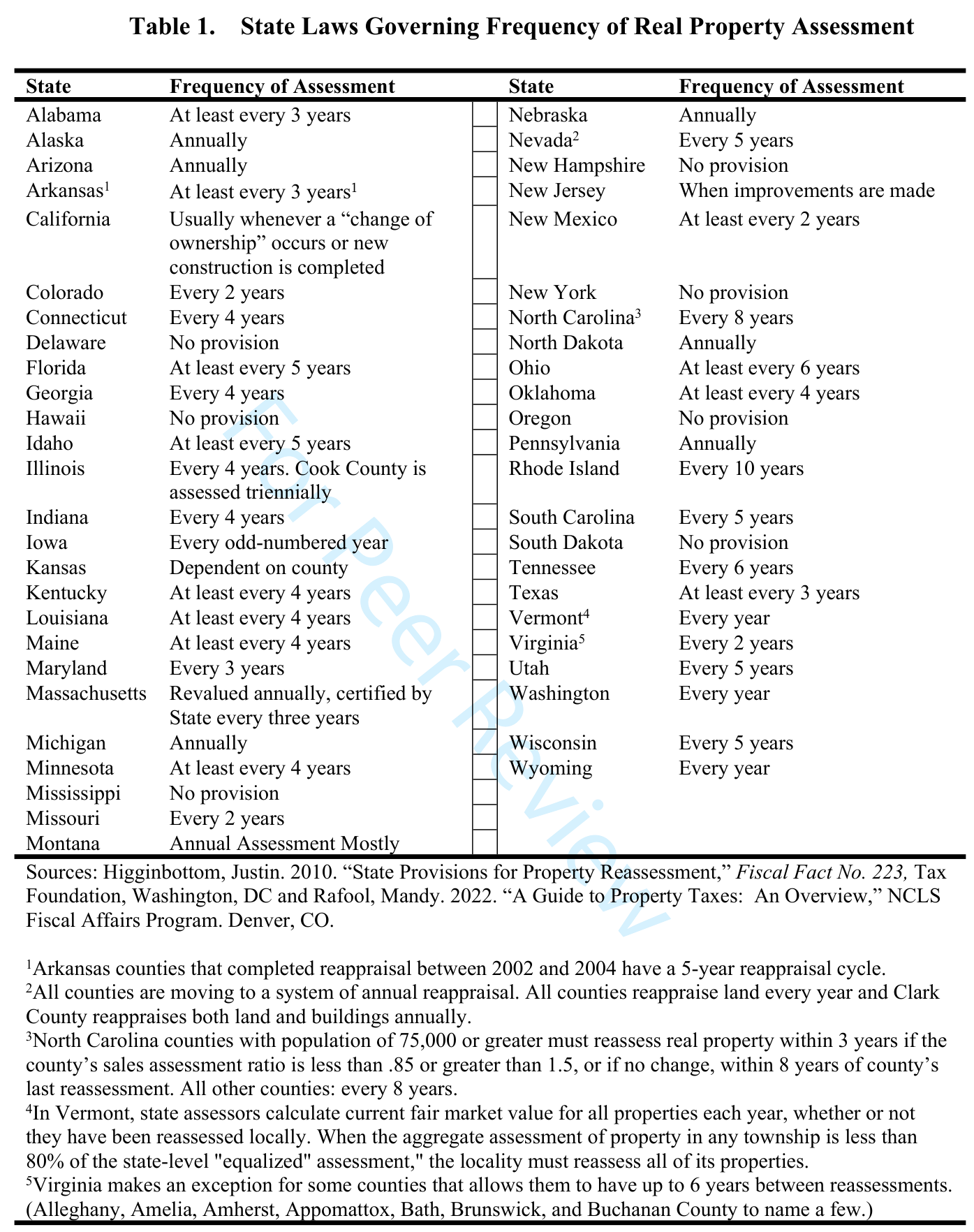In this study we consider another assessment practice, the infrequency of reassessments, that also results in the divergence in property taxes of existing and potential, new property owners. To our knowledge, the possibility that infrequent reassessment might similarly result in “lock-in” effects has been ignored in the literature on property taxation. As can be seen in Table 1, 44 states and the District of Columbia have laws governing how frequently reassessments must occur. While ten states require annual reassessment, the remaining 34 states have reassessment intervals varying in length from two to ten years with 17 states having intervals of four or more years. Two states, Connecticut and Rhode Island, have a ten-year reassessment cycle, and New Jersey only requires reassessment when improvements are made. While the majority of states have a maximum period of time between reassessments (“at least every x years”) some state statutes have a specific length of time or conditions for early reassessment (for example, Maryland). As we show, these extended periods between reassessment can lead to significant differences in the assessments faced by current and new homeowners during periods of high appreciation. And, importantly, in contrast to assessment limits, the periodic reassessment of properties means that the “wedge” in taxes between current and new owners either disappears or is reduced when the property is subject to periodic reassessment independent of a sale. Unlike 20 other states, the Commonwealth of Kentucky does not have a statewide limit on how much assessed property value can increase in a year. Kentucky statute requires that local property value administrators (PVA) revalue every year properties at a _fair cash_ (market) _value_ each year and _examine_ each property no less than every four years.³ In practice, at least in Lexington, distinct neighborhoods are most frequently examined on a four-year cycle and it is following this neighborhood assessment that properties are revalued (reassessed). A household that has lived at a property for three years since the last neighborhood assessment may, particularly in times of high housing appreciation, have an assessment significantly below what a new purchaser with an assessment based on current market value. However, the next year, four years from the previous statute-required assessment, the house will be reassessed, and, if assessed at market value, the incumbent household will have an assessment more comparable to that of a new owner. Thus, as with restrictions on assessments, the gap between neighborhood assessments leads to a difference in tax payments between a current and prospective homeowner. Unlike tax differences arising from assessment limits, this difference disappears or is greatly reduced with the next assessment. In this case, the likelihood that a household sells its house depends on: 1) whether a neighborhood assessment occurs in that year and 2) the magnitude of the difference in taxes based on the assessed value before reassessment and the revised amount following it. Using administrative data from the _Fayette County Property Valuation Administrator (PVA)_, we test these predictions. Based on these data we first find that tax payments can change significantly when neighborhoods are reassessed with a mean increase of over $300 ($2020) and, for the homes with the highest assessments, an increase of over $470 per year with reassessment. Using a difference-in-difference strategy with the neighborhood assessment as the treatment, we find that probability of a sale occurring in the year of reassessment increases by approximately 4.5 percent for the sample and over seven percent for houses in the 25^th - 75^th percentile in assessed value. Alternatively, by estimating the change in taxes with reassessment using two-stage least squares, we find a ten percent change in property tax payments arising from reassessment increases the likelihood of a sale by approximately 3.7 percent and by over seven percent for the homes in the third quartile of assessed value. ## LITERATURE REVIEW There is a large and varied literature on property taxes and, specifically, on the impacts of property tax limits. Numerous studies examine the political and economic motivation for these regulations. For example, Anderson (2006) argues that while property tax limits may serve as a constraint on local government expenditures, these limits also serve as insurance against unexpected increases in personal property tax liabilities. A related motivation for property tax limits that coincides with many of the limits imposed in the 1970’s and early 1980’s is as a “defense” against inflation-induced increases in property tax liabilities (Bowman 2006; Cornia and Walters 2006) or Leviathan governments seeking to maximize revenue (Cutler, Elmendorf, and Zeckhauser 1989). Other studies focus on the impact that property tax limits have on local revenues and expenditures (Bradbury, Mayer, and Case 2001; Lang and Jun 2004). Another strand of the literature on property taxation and property tax limits focuses on the distributional impacts of these limits (Dye, McMillan, and Merriman 2006; Hodge, Sands, and Skidmore 2015; Skidmore, Ballard, and Hodge 2010). While our study is not focusing on the effects of property tax limits on homeowner mobility, it is related to these studies as it explores an institutional aspect of assessment that “locks-in” assessed value for current homeowners. The literature on property taxation and mobility has, for the most part, focused on several “case-study” state-level reforms. Most notably, there are numerous studies on the economic effects of California’s Proposition 13. Enacted in 1979, Proposition 13 reduced the property tax rate to one percent of assessed value, and limited increases in assessments to, at most, two percent per year. However, assessments are set to market value at sale, potentially creating a “lock-in” effect, especially for long-tenure owners in rapidly appreciating housing markets. Several other states, including Massachusetts and Florida, have enacted similar limit on assessments. The empirical approaches employed to examining the effects of property tax limits typically rely on household data and examine household behavior immediately before or after a change in policy. The reliance on household data, while allowing researchers to include household characteristics that may affect mobility, means researchers often have crude measures of mobility and property tax burdens. The focus on the immediate passage of laws also creates potential problems as, in some instances, the effects of these limits may not be seen in the short run. For example, Nagy (1997) finds little lock-in effect from Proposition 13, but others argue that there was little time to find such impacts as Nagy only examines behavior for three years after the law was enacted (Wasi and White 2005). In other instances, the short-run effects may be larger than the long-run effects due to pent-up demand. Ferreira (2010) finds large increases in mobility for Californians over the age of 55 using the 1990 Census, soon after several amendments allowed older homeowners to transfer their property tax savings to another home in California, but these amendments resulted in much smaller effects in the 2000 Census. Hodge et al. (2015) examine the impact of taxable value growth caps on mobility using parcel-level data in Detroit, Michigan and find longer durations of property ownership for those who received greater reductions in their effective property tax rate. Focusing on Florida’s assessment limits, Ihlanfeldt (2011) finds evidence of a lock-in effect for homeowners in single family homes. In contrast, Stansel et al. (2007) find no evidence that Florida’s cap, which is portable across the state, had an impact on tenure. Stohs, Childs, and Stevenson (2001) identify the impact of Proposition 13 on homeowner mobility through comparisons of home sales in selected counties in California with selected counties in Illinois and Massachusetts and finds fewer housing sales in the California counties. Wasi and White (2005), focus on the impact of Proposition 13 on tenure length of owners, employing Florida and Texas as comparisons and using a “difference-in-difference” methodology with microdata on households from the 1970 - 2000 Census of Population and Housing. They find that length of tenure in California increased by 0.66 years or six percent following the passage of Proposition 13. Many lock-in studies clearly recognize the frailties of strictly relying on time series variation to identify the effects of an introduction or modification of these limits. Although the passage of a law that limits property taxation may certainly affect owner mobility, a host of other factors, including changing employment and housing markets, may also matter. Typically, researchers have examined owners in unaffected markets (e.g., housing markets outside of California in the Proposition 13 context), or owners that are differentially affected by the law (e.g., those with high or low tax savings). Approaches that rely on cross-state control groups often suffer from the problem that different property tax systems can be correlated with other underlying characteristics of the state that also affect household mobility.⁴ Moreover, these studies have difficulty controlling for differential trends in housing markets over time as these trends could independently affect mobility and may be correlated with the tax savings.⁵ Approaches that rely on differential tax savings to identify mobility effects often have difficulty in disentangling the causality issues: in appreciating housing markets, longer tenure increases property tax savings, while the empirical approach often estimates the impact of property tax savings on mobility which is highly related to length of owner. The literature discussed above focuses on the lock-in effect resulting from differences in assessments between current owners and purchasers of a property. That this increase in property taxes only arises with a sale effectively makes the increase in property taxes with the change in ownership a real-estate transfer tax. As noted in Slemrod, Weber, and Shan. (2017) 35 states and the District of Columbia apply transfer taxes on residential real estate transactions with a mean rate (2012) of 0.58% but in D.C., the focus of their study, the rate ranged from 2.2 to 2.9 percent. The U.S. is not the only country that applies these transfer taxes, Fritzche and Vandrei (2019) examine transfer taxes in Germany and Eerola et al. (2021) examine them in Finland. Both studies find significant lock-in effects of these transfer taxes and anticipatory changes in the timing of transactions when rates are changed. Zhang and Deng (2023) examine a specific transfer tax in Singapore, a seller stamp duty (SSD). Unique to this tax is the duration-dependence of the tax – the longer the property is held, the lower the tax rate that is applied to sale. Not surprisingly, Zhang and Deng find that higher tax rates and longer “lock-in” periods reduces the probability of a sale. Interestingly, they also find that increases in the lock-in period and tax rates lead some homeowners to lease out their properties. A related literature examines lock-in with respect to housing appreciation and mortgage interest rates (Quigley 1987, Nakagami and Pereira 1991, Ferreira 2010, Chan 2001, and Fonseca and Liu 2023). Evidence from these and other studies suggests that household mobility might be affected by changes in housing prices and mortgage interest rates. Finally, Spreen and Keddington (2023) examine the lock-in effects of short-term (five year) property tax relief to long-tenured (40 years) senior (age 60 and over) homeowners passed in Maryland in 2016 and adopted by some but not all counties. Using both difference-in-difference and regression discontinuity strategies, they find no statistically significant evidence that the property tax relief affected property sales decisions of eligible senior homeowners. Relative to existing work, our study offers several innovations. First, our source of tax assessment variation is transparent and clearly exogenous to the household. Second, we rely on tax assessor data, meaning we measure mobility, tax assessments and housing characteristics far more precisely than typical household-based surveys. Third, any fears about differential housing market trends affecting mobility are reduced as we are examining mobility within a single housing market with our exogenous variation occurring at the neighborhood level. Finally, as we examine behavior over the period 2002 to 2020 concerns about overstating the long-run impact of property taxation due to pent-up demand should be greatly reduced. ## ASSESSMENT-INDUCED TAX DIFFERENTIALS AND THE DECISION TO SELL Here we illustrate how differences in property taxes between existing homeowners and new purchasers can arise and what factors determine the magnitude of these differences. Our parameterization gives some indication of the potential magnitude of how these tax differences and how they may vary over the assessment cycle. As motivation for our empirical work, we provide a simple example of how these tax differences affect the likelihood of a household moving or, equivalently, when there is a sale of property.⁶ ### Determinants of Assessment-Based Tax Differentials To understand the differences in tax payments between a current and potential new homeowner, consider the example of a homeowner who just had their home reassessed at a value of $500,000, equal to the current market value. Then if the assessment cycle is four years and the homeowner stays in the house until the next reassessment, with a two percent property tax rate, her tax payment for each of the next four years is $10,000. Now, with an annual appreciation rate of 7.5 percent, someone purchasing the house the year following the neighborhood assessment would pay and be assessed at the current market price of $537,500, paying annual taxes of $10,750 for the three years until the next neighborhood assessment — $750 more per year than the current owner. 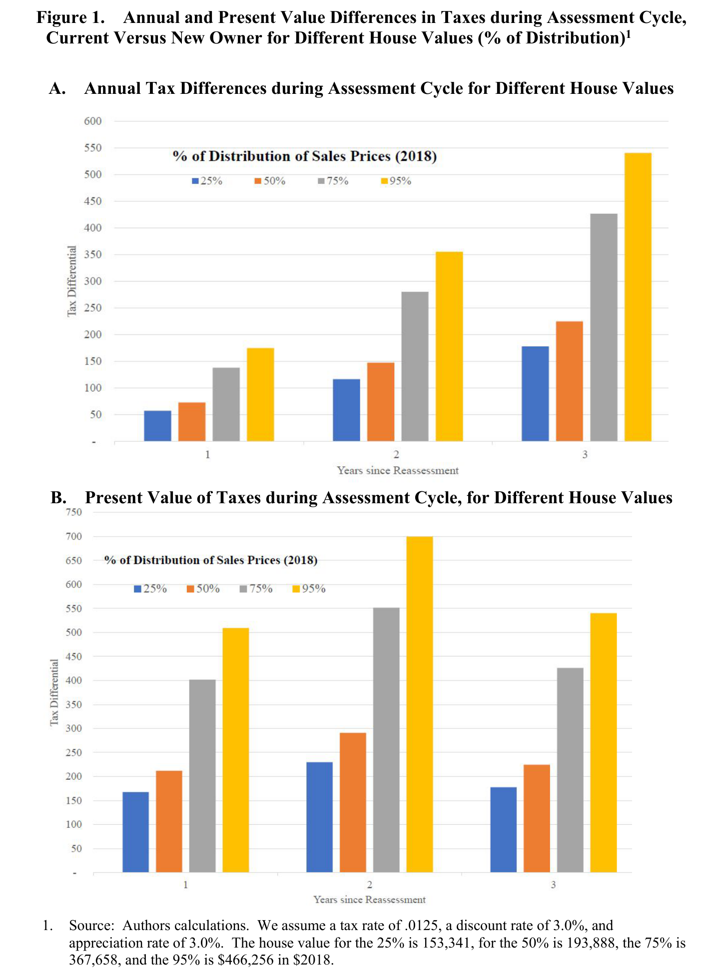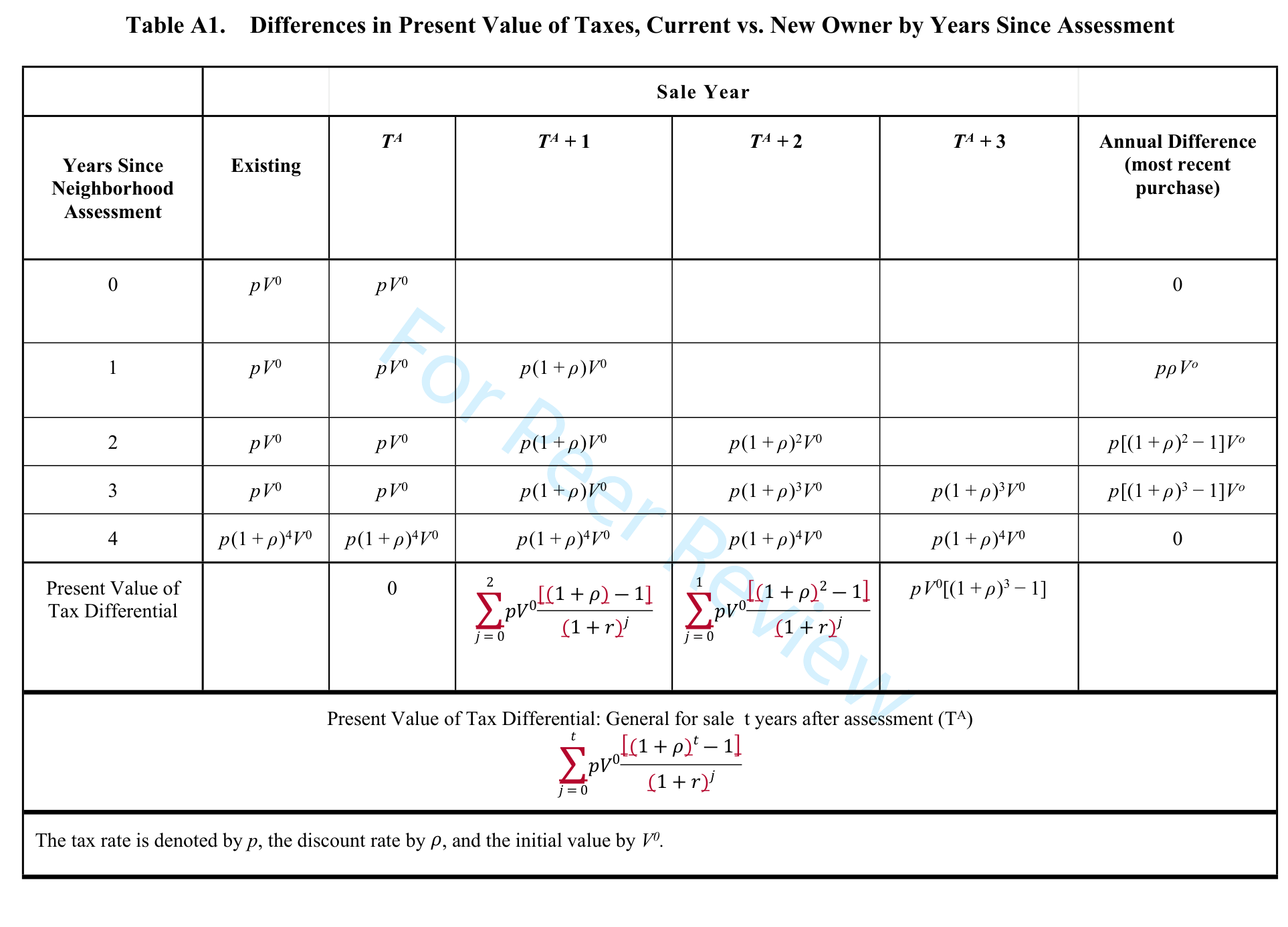As seen in Figure 1a, the difference in annual tax payments between current homeowners and potential purchases continues to grow until the next neighborhood assessment. In this figure we show this difference in annual tax payments based on the years since assessment for homes at the 25^_th_ , 50^_th_ , 75^_th_ and the 95^_th_ percentiles of sale value which, in 2020 (at $2020), are $153,341, $193,888, $367,658, and $466,256. We assume a tax rate of 1.25 percent with both the appreciation and discount rate set at three percent.⁷ Figure 1b reports the differences in the present values of the tax payments. While the greatest annual tax difference is in the third year following assessment, the greatest difference in the present value of taxes is found in the second period.⁸ ### Assessment-Based Tax Differentials with Incomplete Reassessment Kentucky law states that properties are to be assessed at “fair cash value” and, unlike other states, there are no statutory limits on how much assessments can increase. However, the tenure of a property owner can have a significant impact on the assessed value of her property, suggesting that properties are not necessarily assessed at “fair cash value” when a neighborhood assessment is done. 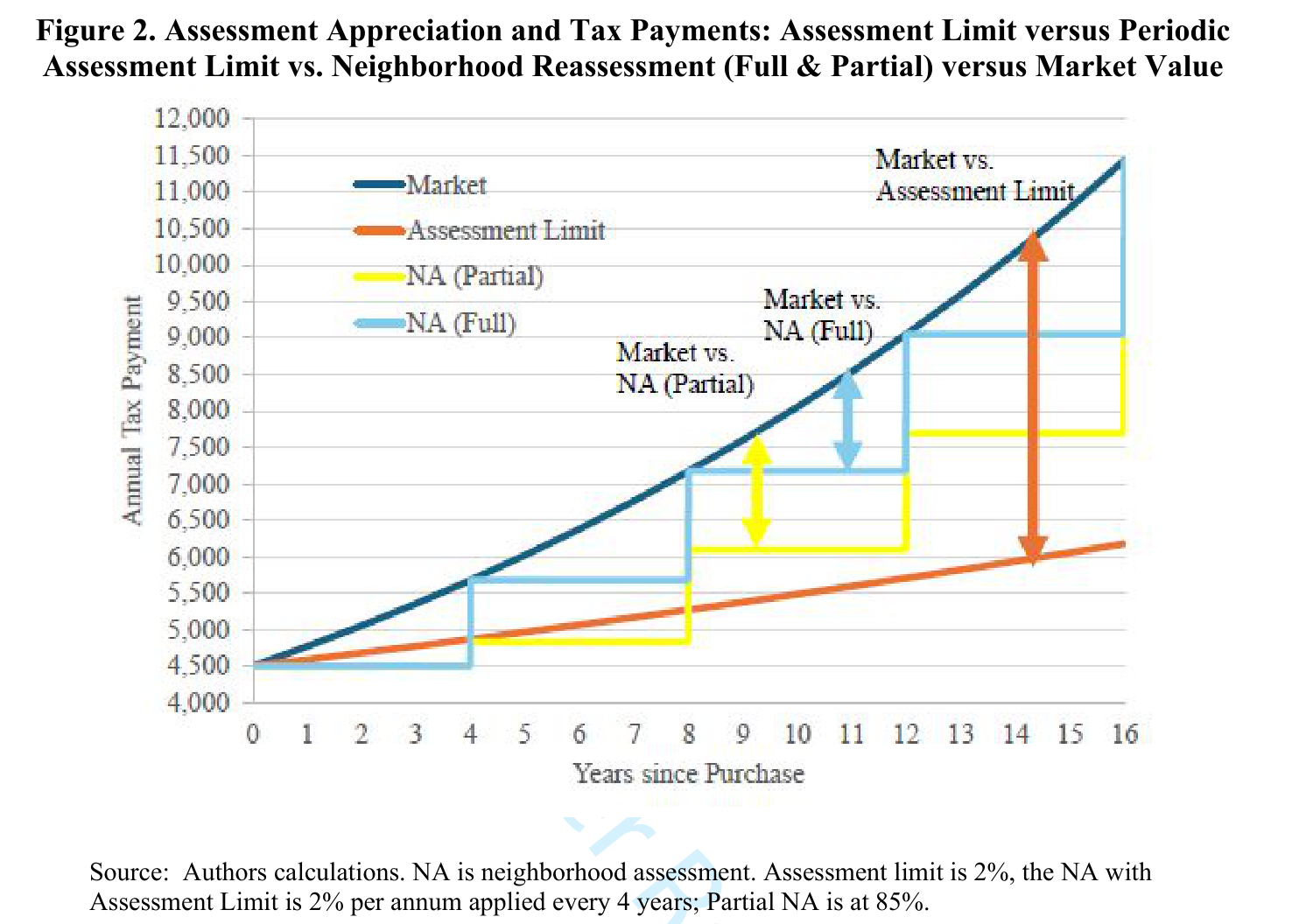Figure 2 compares the difference in tax payments over multiple assessment cycles for four alternative assessment strategies: annual assessment at market value, annual assessment with an assessment growth limit of two percent, assessment every four years at 85 percent of market value, and assessment every four years at full market value. Note that the “wedge” between tax payments for annual reassessment at full market value and those when assessment limits apply only increases over time. However, when reassessment is on a cycle, the wedge increases during the cycle but decreases or disappears every four years. Thus, while there is a continuous increase in the tax wedge between current and new homeowners when there is an assessment limit, there is a discrete “jump” in taxes for current homeowners every four years when reassessments are on a cycle. It is this discrete jump in taxes for a current homeowner and how it might influence the sale of their home that is the focus of our empirical analysis. ### Timing of Sales with Known versus Uncertain Reassessment The example of the property tax differences between existing and new homeowners discussed above presumed, following Kentucky Statute, that an inspection and subsequent reassessment occurs every four years. As we shall see later, while this four-year cycle of neighborhood reassessments seems to have been followed for in the years before 2010, reassessments were less frequent and did not follow any obvious pattern after 2010. Of course, that reassessments did not occur on a four-year cycle, may be partly explained by the limited appreciation of properties during and shortly after the Great Recession. But, as becomes apparent with our calculation of differentials between assessed and market values, the limited appreciation in property values does not fully explain all the apparent deviations from the four-year cycle. How, then, might uncertainty in neighborhood reassessments affect the decision of homeowners to sell? To the extent that homeowners make the decision of whether to sell based on current annual differences in tax payments, the timing of the next neighborhood reassessment is irrelevant. However, if their decision is based on the present value of the current and future tax savings, the timing of the neighborhood reassessment matters.⁹ Regardless of whether a neighborhood assessment is expected or not, the occurrence of the reassessment is likely to result in a distinct and discrete increase in a homeowner’s taxes will that is likely to persist for several years. The realization that her taxes have increased and how much they did may change the homeowner’s incentive to remain in her current home. The focus of our empirical work is to examine how these neighborhood assessments¹⁰ affect the probability of a sale. ### The Decision to Move To illustrate the impacts of property tax assessments on moving, consider a simple model in which a household, at any time _t_, has their own valuation of their home, _V_⁰(_t_), and is aware of the market valuation at that time, _V_(_t_). There is also a moving cost of _M_(_t_). Initially, assume that there is no tax difference between a current and a potential new homeowner with assessed value equal to market value for both. Then the current homeowner will sell if: **Equation (1):**

π (t) = V (t) - V^{0} (t) - M (t) > 0 .

However, because assessed values lag market values, there is differential tax treatment between the current and a new owner and there will be a change in ownership only when: **Equation (2):**

\tilde{π} (t) = V (t) - V^{0} (t) - M (t) - Δ P (t) > 0,

the bid of the potential buyer,

V (t)

, exceeds the valuation of the current owner,

V^{0} (t)

, her moving costs,

M (t)

, and her tax advantage,

Δ P (t)

. Then introducing a random component into (2) enables us to relate the tax wedge between current and new homeowners to the probability of a current homeowner moving (selling their house) -- a link to our estimation. We assume that the valuation of the current owner reflects the market but has an idiosyncratic (randomly distributed) component, or

V^{0} (t) = V (t) - ε_{t}

. Then substituting for

V^{0} (t)

in (2) we obtain: **Equation (3):**

\tilde{π} (t) = ε_{t} - (M (t) + Δ P (t)) > 0 .

It follows from (3) that if

\tilde{π} (t) > 0

, or equivalently if

ε_{t} > ε_{t}^{*} \equiv M (t) + Δ P (t)

, the household will move with the probability that it moves at time

t

given by

P (ε_{t} > ε_{t}^{*})

. Then, as

ε_{t}^{*} \equiv M (t) + Δ P (t)

ε_{t}^{*}

increases in both the tax and appreciation rates, meaning that the likelihood of a sale is lower between neighborhood assessments than in the year of a neighborhood reassessment or immediately after. ## DATA Our primary source of data is from the Property Valuation Administrator (PVA) in Lexington-Fayette County, Kentucky. We obtained these data for virtually every parcel in the county. They are unique in several respects. First, they are unusually detailed. In addition to reporting current tax assessment, parcel identification, street address, house and lot characteristics, all tax assessments from 2002 onward are available. Legal transactions (such as arms-length sales, quit claim deeds arising from divorce, foreclosure proceedings, etc.), along with relevant dates, parties, and prices, are also recorded. Second, each parcel is classified into one of 344 neighborhoods in Fayette County. As shown below, this is vital to our identification strategy, because parcels are assessed at different times based on their neighborhood. Finally, access to the data is unusually open. The detailed data we utilize is freely available at the website www.fayettepva.com. 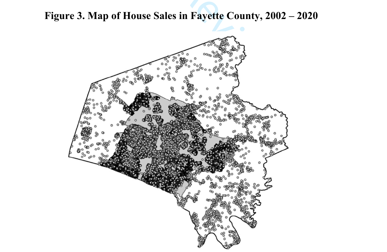Our focus is on single-family homes, and we restrict the sample to only include arms-length transactions. Ultimately, we have a sample of single-family residential homes located in 344 neighborhoods. Figure 3 plots these parcels in Lexington. On the map, the shaded area is the Urban Service Area where most of the development of single-family homes occurs and where city water and sewer are provided. Outside of the urban service area is the rural service area, without city water and sewer and where development is more restricted. Most of this area is agricultural with horse farms constituting a large share of the land. In our analysis, we separately examine urban and rural service areas. ### Tax Assessment in Lexington and Identification Strategy In Lexington, there are seven tax districts for single-family residential homes with modest variation in the tax rates among them – ranging from 1.10% to 1.28% of assessed value in 2020. The variation arises in large part because some neighborhoods rely on private garbage collection, street cleaning and street light maintenance. Newer neighborhoods cannot opt-out of having these services being publicly provided and if a neighborhood switches from private services to public services, that switch is irreversible. Of the homes in our sample, almost seventy percent receive full public services and pay the highest tax rate. Kentucky law (KRS.132.690) states that each parcel will be assessed annually by the PVA at its fair cash value in accordance with standards prescribed by the Revenue Cabinet. In addition, property will be physically examined no less than once every four years by the PVA. In practice, houses in Fayette County are reassessed in the tax year following a sale. As well, neighborhood assessments are usually updated once every four years though this may not mean that assessments change. If properties in a Lexington neighborhood, in aggregate, have unusually high rates of appreciation or depreciation, then neighborhood assessments may occur more than once every four years though this occurs infrequently. 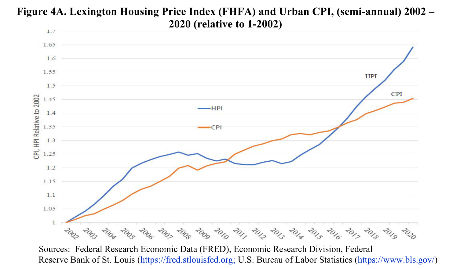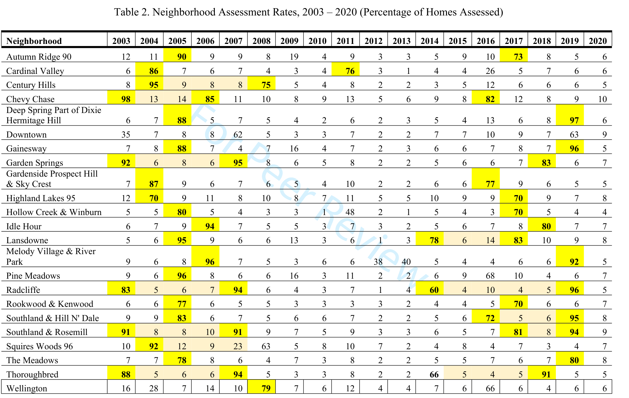Table 2 reports the share (percentage) of houses assessed for 24 large neighborhoods from 2003 to 2020 with the cells highlighted in dark yellow denoting neighborhoods with a high percentage (70%+) being reassessed, our criterion for a neighborhood assessment. While approximately one-quarter of homes in Fayette County appear to be assessed from 2003 – 2008, from 2009 – 2013 only one neighborhood, Cardinal Hill in 2011, met our criterion having a neighborhood assessment. That there was very little assessment from 2009 to 2013 is consistent with housing prices not increasing during this period and, in fact, falling for several years as can be seen in Figure 4a. In 2014, neighborhoods again appear to be subject to assessments consistent with housing prices rising, as seen in Table 2. For most cases, it is clear which neighborhoods are being reassessed and which neighborhoods have a few properties reassessed because of transactions or structural changes to the property. Our identification strategy – an important contribution of our paper – is motivated by this table. In older, more established neighborhoods, it is easy to see when wholesale assessments occurred (at least if property values are appreciating). The fact that houses in one neighborhood are assessed in a given year, whereas houses in another nearby neighborhood are not, creates plausibly credible variation in property tax burdens for individual homeowners. This allows us to construct a difference-in-difference estimator of the impact of assessment on property sales, using the differential timing of assessments across neighborhoods to estimate this effect. Several comments about our approach are in order. First, we are ultimately inferring that a neighborhood was subject to assessment based on observed changes in assessments in that neighborhood. Some neighborhoods were certainly subject to assessment under Kentucky law, but their assessments were not revised when appreciation was low or even negative. Our procedure will have difficulty in detecting these neighborhoods and assessment years. In Table 2, the years for which the neighborhood was subject to a _binding_ neighborhood assessment are highlighted in yellow. Those neighborhoods for which we could identify a four-year interval between assessments are in bold as well. An example of a _binding_ assessment is found for the “Cardinal Valley” neighborhood – in 2004 it had a wholesale assessment (86% of parcels), however only a trivial amount of assessment occurred there in 2008. Put differently, our approach detects binding neighborhood assessments, but not non-binding neighborhood assessments.¹¹ Second, as mentioned, we define a threshold of 70 percent in a neighborhood as a binding, scheduled neighborhood assessment.¹² Note that assessments primarily occur for two main reasons: “wholesale” neighborhood assessment and as a result of individual property sales (which is our outcome of interest). The assessment percentage in Table 2 includes both. While four years is a maximum interval between assessments, as can be seen in Table 2 several neighborhoods (those not in bold) were assessed in a three-year interval or on an interval with a length we cannot identify. This is an issue that we address empirically. 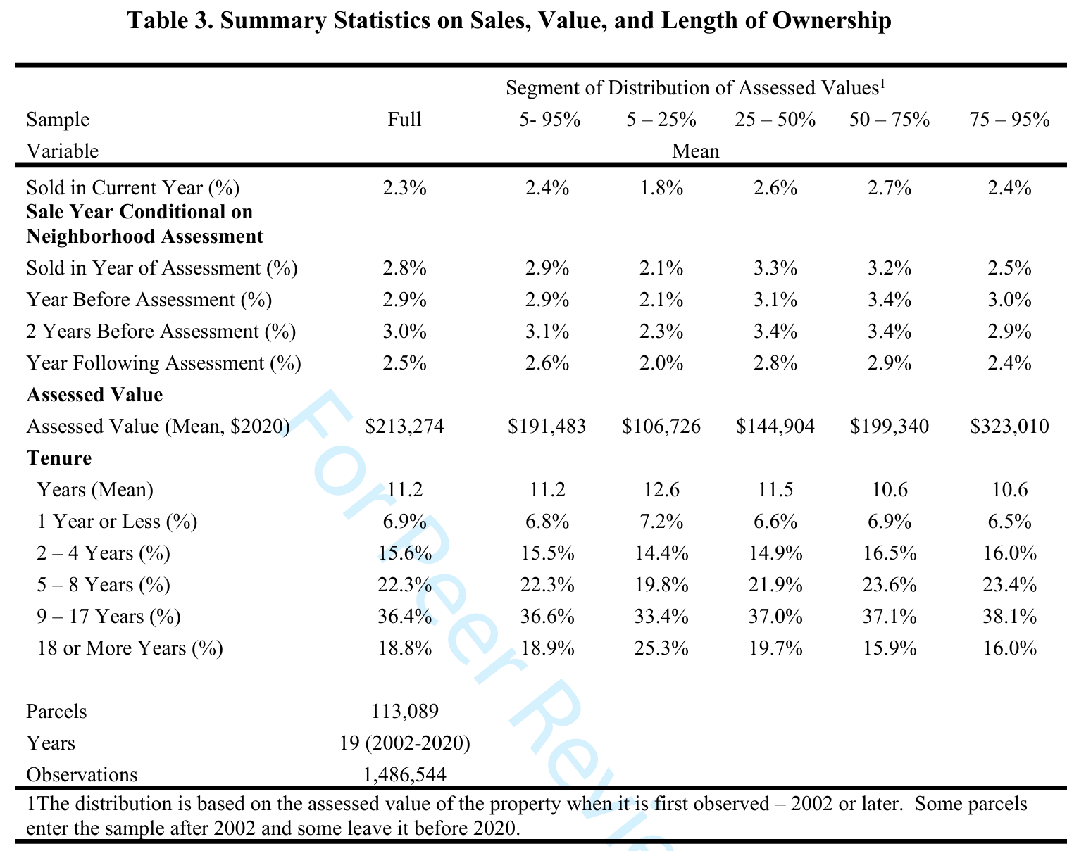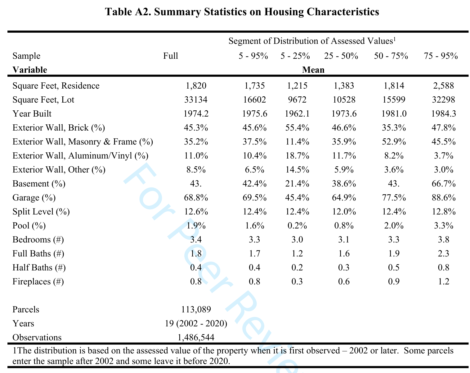### Summary Statistics Table 3 provides summary statistics on sales, assessed values, and tenure length for the sample of single-family dwellings we utilize in our estimation. Table A2 in the Appendix provides additional summary statistics on the characteristics of the dwellings, other variables employed in our estimation strategy but not our focus. From Table 3 we can see that approximately 2.3 percent of houses are sold each year. We also consider the distribution of sales conditional on the house being in a neighborhood assessed in that year. Then from the table we see that the percentage of houses sold in the year a neighborhood is being assessed is higher than when no neighborhood assessment occurs (sold in current year). The mean assessed (fair cash) value for our sample of houses was $213,274 ($2020). As much of our empirical analysis employs sub-samples of the properties based on the average assessed value in the neighborhood, we provide additional information about the distribution of assessed values. Mean tenure length was 11.02 years with approximately seven percent of households residing in their house less than a year and almost 20 percent in their house for over 18 years. 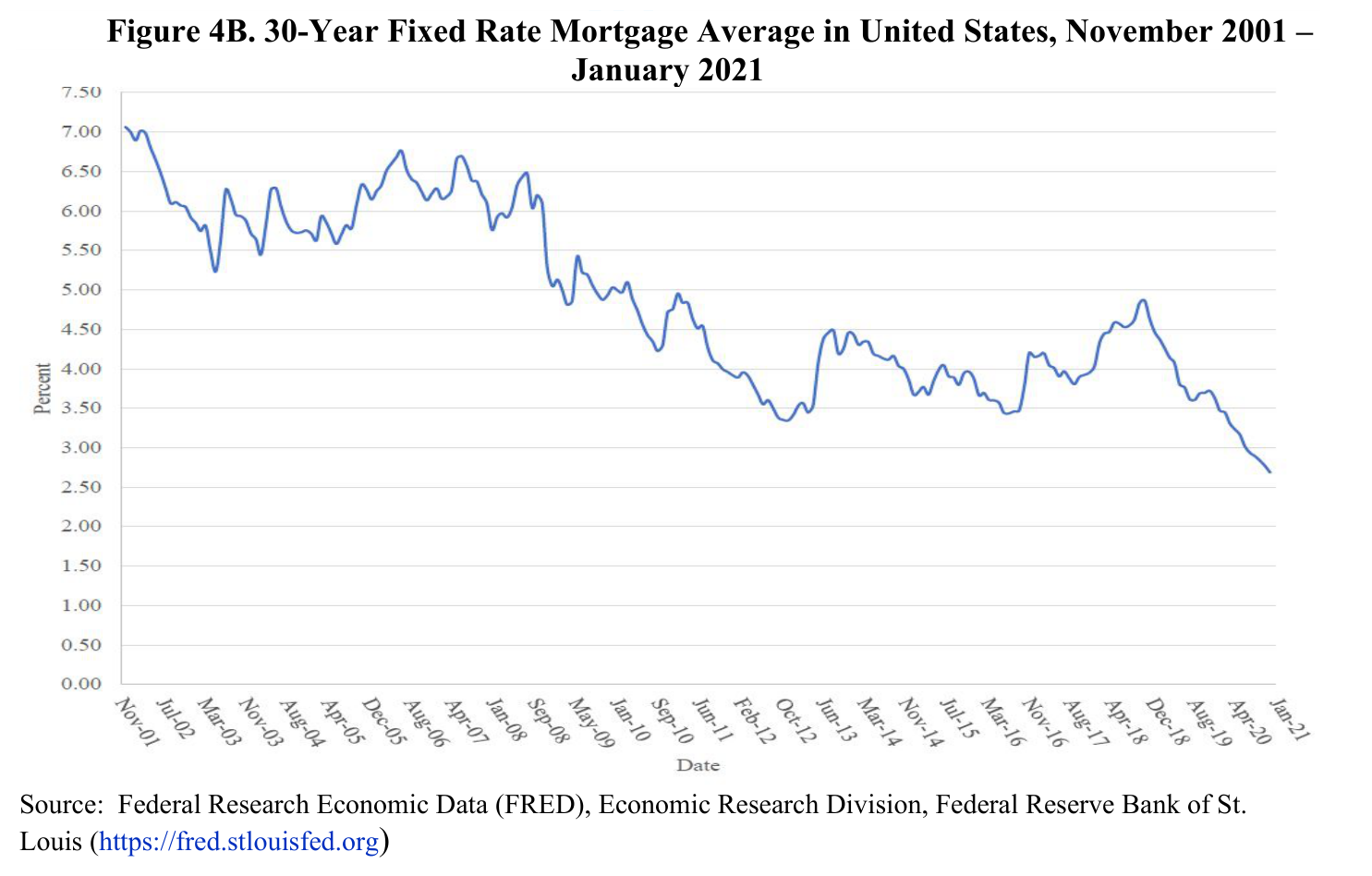### Housing Appreciation and Mortgage Interest Rates Numerous studies have examined how mortgage interest rates and household appreciation might affect household mobility and lock-in. In Figure 4a, we report the FHFA housing price index for the Lexington metropolitan area. As is evident from the figure, housing prices appreciated from January 2002 to April 2008 by 26 percent, an annual rate of approximately four percent, then were relatively flat and falling until January 2015. From January 2015 to January 2021 housing prices increased by 34 percent, an annual rate of five percent. For the entire period, 2002 to 2020, housing prices increased by an average of 2.82 percent per year. In Figure 4b, we report the monthly average 30-year fixed mortgage rates for the U.S. during this period. Rates are variable but generally decrease during this period. While these fluctuations in housing prices and mortgage interest rates may affect mobility, they are not the focus of our study, and we address these concerns in our estimation through time fixed effects. ### The Magnitude of Tax Differentials and Sales vs. Assessment Appreciation We expect wedges in tax payments between current and potential purchasers to arise due to intermittent reassessments with these wedges disappearing when properties are reassessed. We explore the magnitude of these tax wedges in our data and examine the extent to which changes in taxes on a property might differ when the reassessment arises due to a property sale and when it arises due to a neighborhood reassessment. 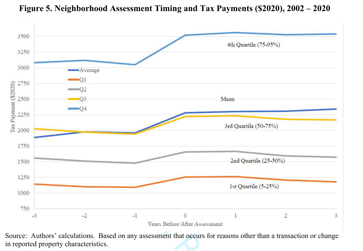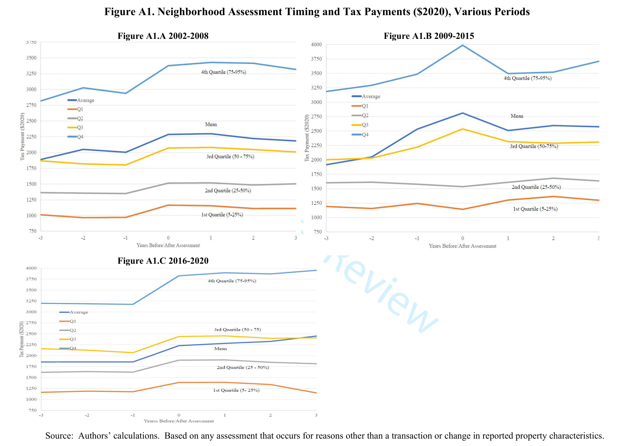### Neighborhood Assessment Timing and Tax Payments Figure 5 plots the change in tax payments, by quantile of assessed value and the mean, that arises when properties are reassessed as a result of a neighborhood assessment. As the assessment only changes at time zero, the taxes, in $2020, only vary at the other periods due to changes in the CPI. As seen in the figure, the mean increase in taxes with reassessment is approximately $320. Not surprisingly, the largest increase in taxes, $471 on average, occurs for the most expensive houses. Figure A1 shows how these changes in tax payments vary for the periods 2002 – 2008, 2009 – 2015, and 2016 – 2020. ### Sale Price vs. 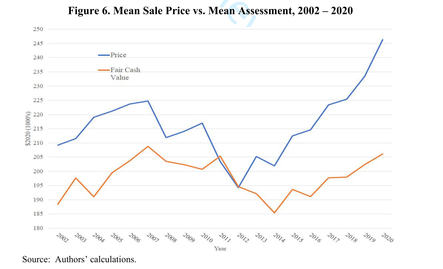Assessment Appreciation Figure 6 plots the time series of sale price and assessment (fair cash value), by quantile and the mean ($2020). The mean sale price exceeds mean assessment in every year except for 2011 and 2012. 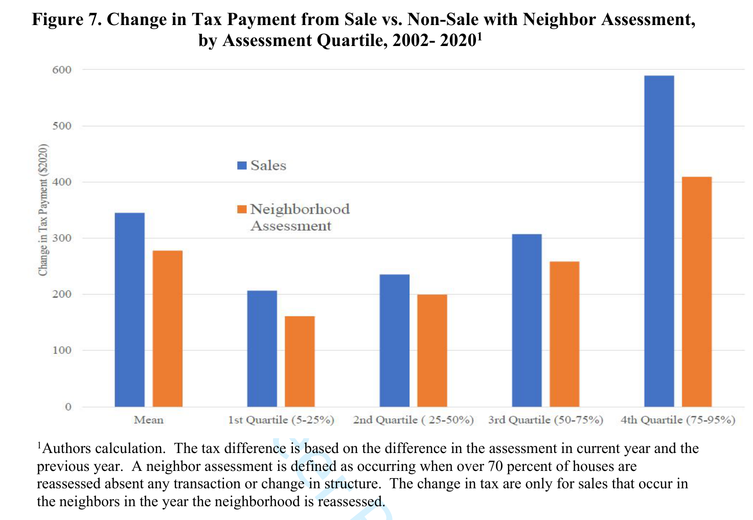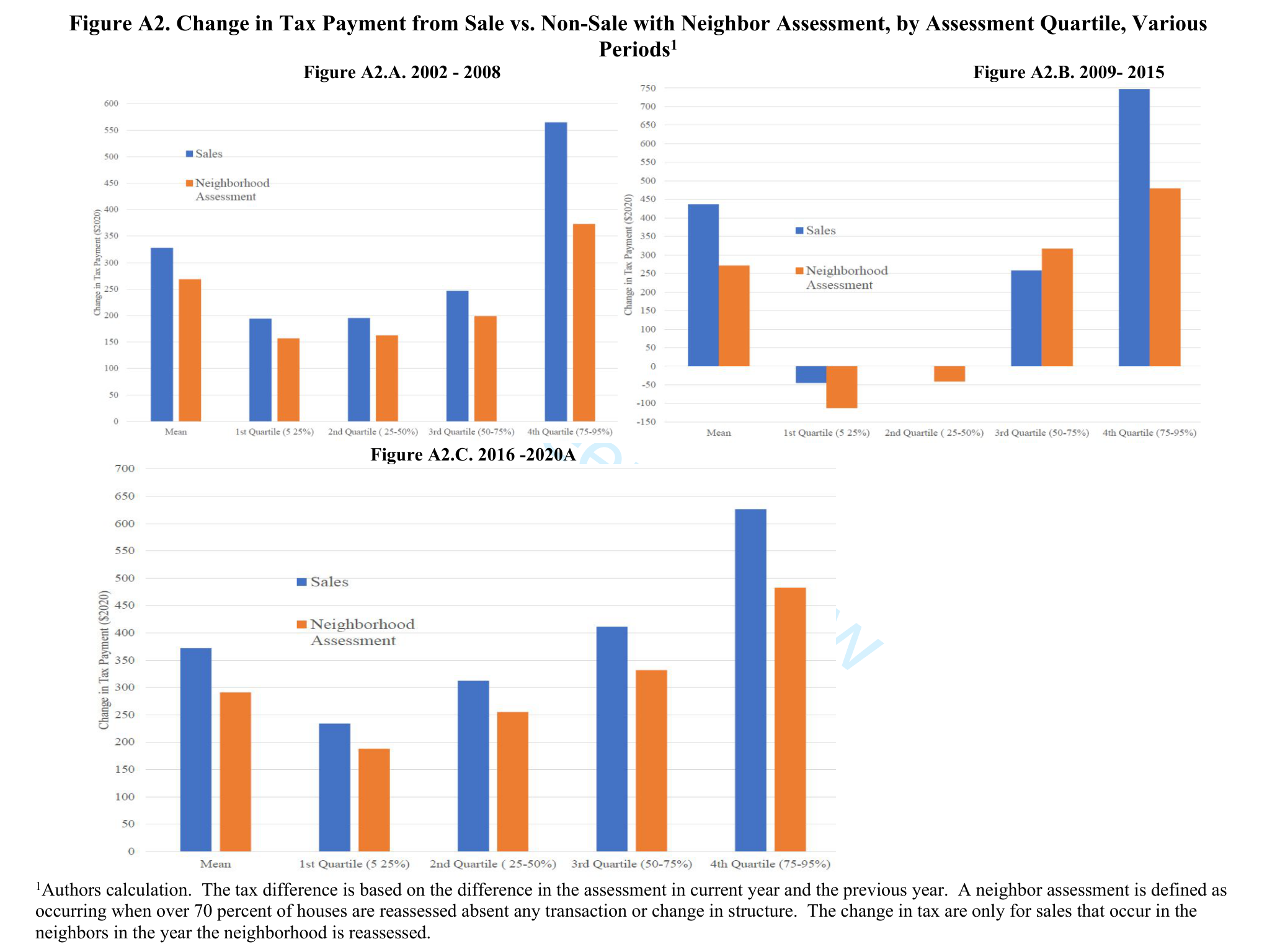Sale prices fell more than assessments during the recession (2008 to 2012) but grew at a faster rate following it. In Figure 7, we compare the change in tax payments for houses that are reassessed, but not sold, during a neighborhood reassessment to houses that were sold in reassessed neighborhoods in the same year by assessment quantile and mean. The difference in taxes for both groups is based on assessed value in the year of assessment relative to the preceding year’s assessed value. For houses that are sold during the year, the practice in Lexington is to set the assessed value equal to the sale price. For houses that are not sold, the assessed value only changes if the neighborhood is reassessed or there are structural changes in the property. The mean change in taxes for houses that were not sold but were reassessed was $278 while the mean change for houses that were sold was $345, 125 percent of the change in taxes from reassessment or $67. The greatest difference in tax payments, in both absolute and percentage terms, is for the highest value homes (4^th quantile) with houses that were sold having a tax change of $180 or 145 percent of those that were reassessed in a neighborhood reassessment. For the lowest quintile, the tax increases for sold houses were 28 percent higher than those reassessed without sale while houses sold in the second and third quintiles were 18 percent higher. Figure A2 provides these tax differences for each of the periods 2002–2008, 2009 – 2015, 2016 – 2020. ## EMPIRICAL FRAMEWORK AND IDENTIFICATION STRATEGY There are a few well-recognized empirical problems in the lock-in literature that make it challenging to estimate the causal effect of property taxes on mobility. As Shan (2010) notes, property taxes are likely to be endogenous to moving decisions, and net property tax burdens are certainly measured with error. Owners who pay high property taxes (and consume higher levels of services) may have different mobility rates than owners who pay low property taxes. For example, homeowners with children may choose to live in areas with high property tax levels if those taxes are used to fund public schools, and these families are also likely to have lower mobility rates than other households.¹³ The goal of most researchers has been to find an exogenous source of variation that affects the net property tax burden but is otherwise uncorrelated with latent mobility. In our case, the fact that most parcels are assessed every four years, and on a staggered basis, provides exogenous variation in both gross and net tax burdens. ### Assessment As discussed, the extent of “lock-in” depends on the extent of the expected increase in assessed value and, therefore, property taxes due to automatic assessment. As also discussed, if households with longer tenure lengths might be assessed at levels below market value, the tax wedge between current and new owners should increase with tenure increasing “lock-in.” To determine the extent that both tenure and automatic assessment affect assessed property value we estimate a regression of the form **Equation (4):**

LN (V_{i n t}^{A}) = γ_{0} + γ_{1} N A_{n t} + γ_{2} T e n u r e_{i n t} + γ_{4} \ln {(\overset{―}{H P I})}_{t} + γ_{4} Y_{n t}^{N A - 1} + μ_{i n} + π_{t} + ε_{i n t}

where

V_{i n t}^{A}

is assessed property value of parcel (house)

i

in neighborhood

n

in year

t

N A_{n t}

is a dummy variable equal to 1 if a neighborhood was assessed in year

t

T e n u r e_{i n t}

is the length of time the current homeowner has been in the home,

\ln (\overset{―}{H P I})_{t}

is the average HPI for Lexington from year

t - 4

to year

t

, and

Y_{n t}^{N A - 1}

is years since last reassessment. The terms

μ_{i n}

is a dummy variable (fixed effect) for the parcel and

π_{t}

is a time fixed effect with

ε_{i n t}

the error term. The employment of a parcel fixed effect combined with the invariance in housing attributes obviates the need to include housing characteristics in this and our other regressions but does limit our sample to properties that are sold at least twice during the period of our sample, 2002 to 2020. ### Neighborhood Assessment and Mobility To determine the relationship between the probability of a home selling and whether the neighborhood assessment occurred in the same year we estimate the model, **Equation (5):**

S a l e_{i n t} = β_{0} + β_{1} N A_{n t} + μ_{i t} + π_{t} + ε_{i n t}

where

S a l e_{i n t}

equals 1 if a home sold in year

t

with the other terms as defined for (4). While we can interpret (5) as a difference-in-difference (DID) model with the neighborhood assessment (NA) being the treatment, there are few distinctions with the standard model. First, unlike the standard model we do not have a term NA\*Post, analogous to the term Treat\*Post in the standard DID as in our case, the treatment, a discrete revision of the assessment, is expected to primarily affect sales in the year of the reassessment and not in the following years. Second, as all neighborhoods are reassessed at different times, we do not have a “control” that has never been treated, raising concerns about how to interpret our DID estimates (Goodman-Bacon 2021). 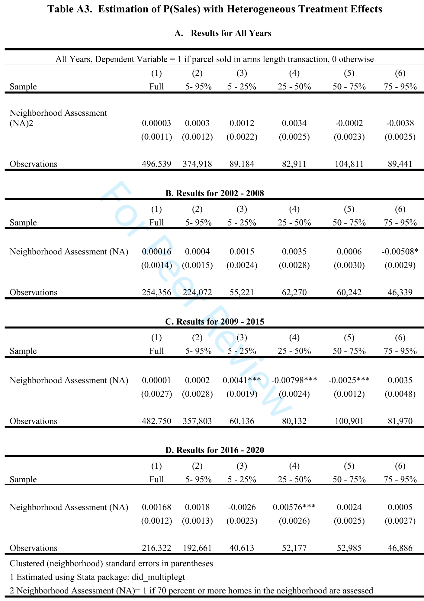Finally, like many studies, we employ two-way fixed effects (neighborhood and time) with the underlying assumption that the effect of the neighborhood assessment is constant over time (De Chaisemartin and D’Haultfoeuille 2020). In Table A3, we report the results of estimates that relax some of the standard assumptions of a DID. As an alternative, we also estimate an equation of the form. **Equation (5′):**

S a l e_{i n t} = β_{0} + β_{1} A_{n t}^{20 - 40} + β_{2} A_{n t}^{40 - 60} + β_{3} A_{n t}^{60 - 80} + β_{4} A_{n t}^{80 +} + μ_{i n} + π_{t} + ε_{i n t}

where

A_{n t}^{x - y}

equals 1 if the percent of houses assessed in neighborhood

n

in year

t

is between

x

and

y

. ### Tax Change and Probability of Sale Our final set of estimates involves a two-stage procedure to first estimate the change in taxes from the previous year,

(Δ T_{i n t})

, associated with a neighborhood assessment,

(N A_{n t})

, accounting for whether the property was reassessed by neighborhood assessment or sale. In our second stage, we estimate the probability of a sale as a function of the change in tax as predicted from the first stage. The first stage is: **Equation (6a):**

\ln (Δ T)_{i n t} = δ_{0} + δ_{1} N A_{t} + ϕ_{i n} + τ_{t} + ε_{i n t}

where

ϕ_{i n}

τ_{t}

, and

ε_{i n t}

are the parcel fixed effect, the time fixed effect and the error term. The second stage is: **Equation (6b):**

S a l e_{i n t} = λ_{0} + λ_{1} \ln (\hat{Δ T})_{i n t} + χ_{i n} + π_{t} + ω_{i n t}

where

\ln (\hat{Δ T})_{i n t}

is the predicted change in taxes from the first stage and

χ_{i n}

π_{t}

, and

ω_{i n t}

are the analogs to

ϕ_{i n}

τ_{t}

, and

ε_{i n t}

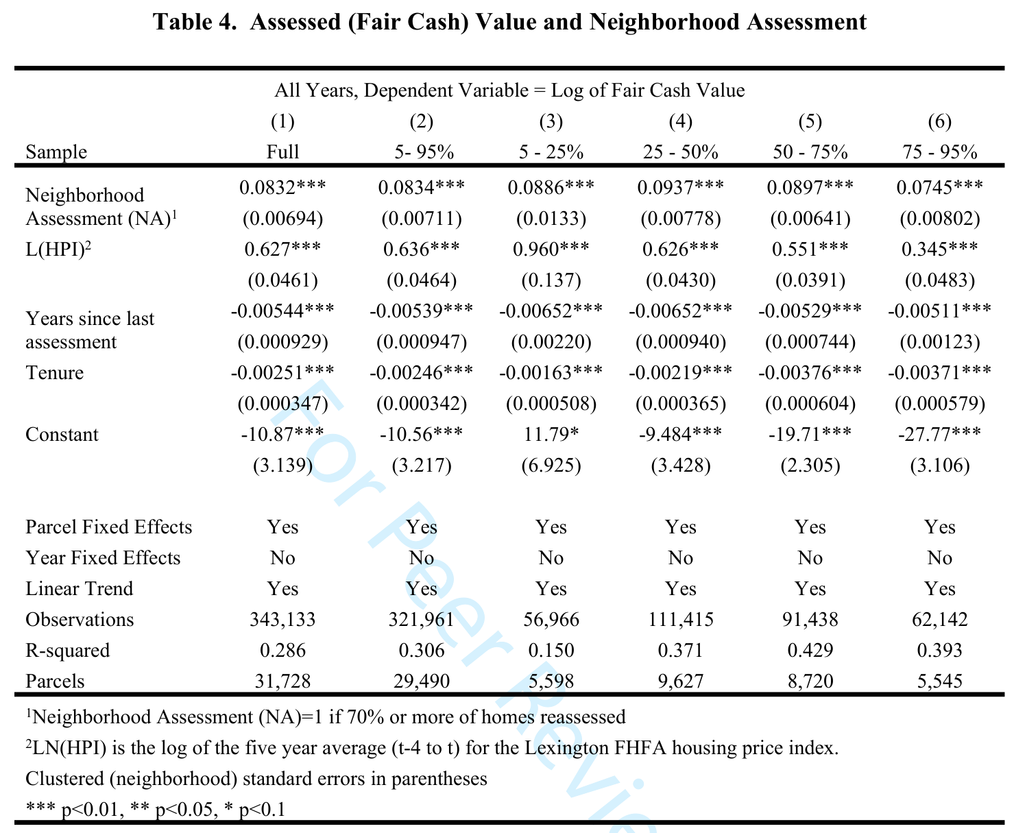
in (6a). ## RESULTS In all tables, we report the results obtain from estimating using the full sample, as well as the results using a trimmed sample of houses that are in the five to ninety-five percentage range of assessed values and using the four quartiles of assessed value.¹⁴ ### Tenure and Assessment Table 4 reports our estimates of (4), the relationship between the log of assessed (fair cash) value and neighborhood assessment as well as the _HPI,_ years since last assessment, and homeowner tenure length. As seen in the table, the coefficient on neighborhood assessment ranges between .0745 to .0937 across our subsamples which reflects an average increase in assessed value of 7.45 to 9.37 percent. The coefficient on _L(HPI)_ ranges from .345 for the highest value houses to .960 for houses in the lowest quartile. As we include _HPI_ as a log then the coefficient on _L(HPI)_ is the elasticity of assessed value with respect to _HPI._ Changes in _HPI_ are almost fully capitalized into assessed values for houses in the lowest quartile but only about a third of the increase in _HPI_ is reflected in higher assessments for the highest quartile of houses. Somewhat surprisingly, the time since the last assessment lowers the assessment, perhaps reflecting delays in assessments for neighborhoods or times with less appreciation. Finally, as we might expect, homeowner tenure length reduces the assessed value with homeowners having the average tenure of 11 years having assessments of approximately 2.7 percent lower than new homeowners. 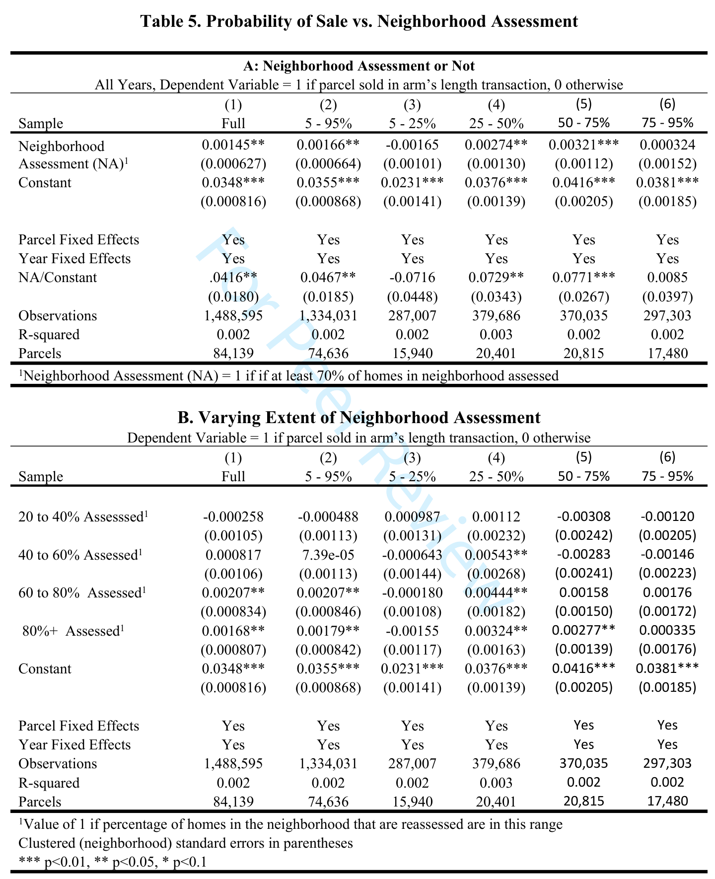### Assessment and Mobility In Table 5A we report estimates of (5), the relationship between a sale of a property and a neighborhood assessment. Interpretation is perhaps simplest by considering the row NA/Constant, the coefficient on neighborhood assessment (NA) divided by the constant. 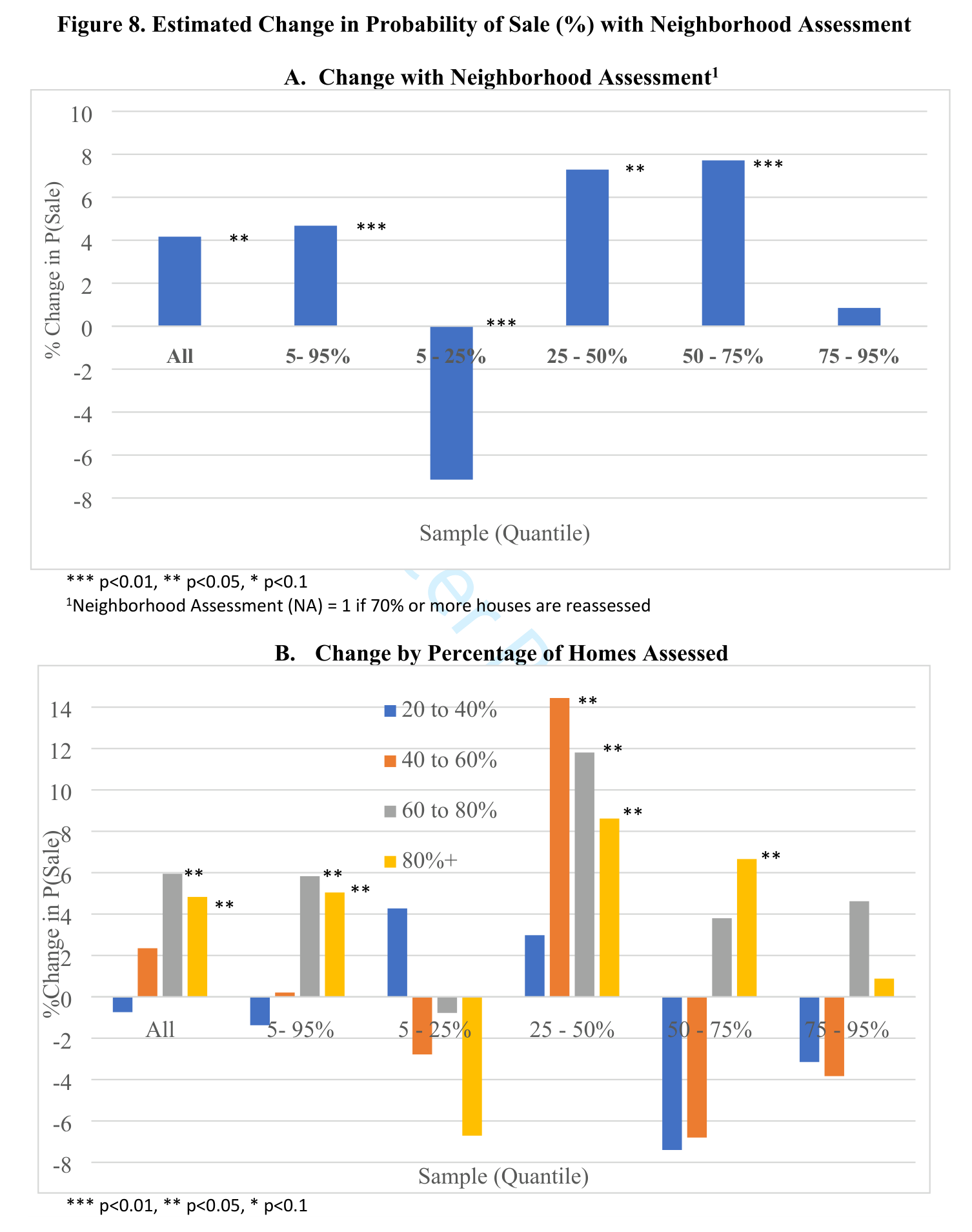This coefficient multiplied by 100 gives the estimated percentage change in the probability of sale resulting from a neighborhood assessment. This is depicted in Figure 8A as well. Relative to those homes not facing a neighborhood assessment, the probability of a sale increases by about four percent for the full sample, with the greatest increases of over seven percent for houses in the second and third quartiles. Sales in the first quartile decrease in a year with a neighborhood assessment by over seven percent while there is no significant effect on sales in the highest quartile. In Table 5B and Figure 8B we report the results when we include multiple categories for the percentage of homes reassessed in neighborhood. For the full sample and the sample of the 5 – 95% assessed values, only assessment rates above 60 percent have a significant effect on sales. Interestingly, there is a higher likelihood of sale for assessment rates in the 60 – 80 percent range than when rates exceed 80 percent. However, this relationship varies dramatically among the quartiles – there are no significant effects in the lowest or highest quartiles, consistent with what we found with the single measure of neighborhood assessment. However, for the second quartile, the percentage increase in sales is high and statistically significant for all categories above 40 percent with the largest increase in sales for assessment rates in the 40 – 60% range and descending as rates increase. For the third quartile, only for rates of assessment above 80 percent was there a statistically significant increase in sales. 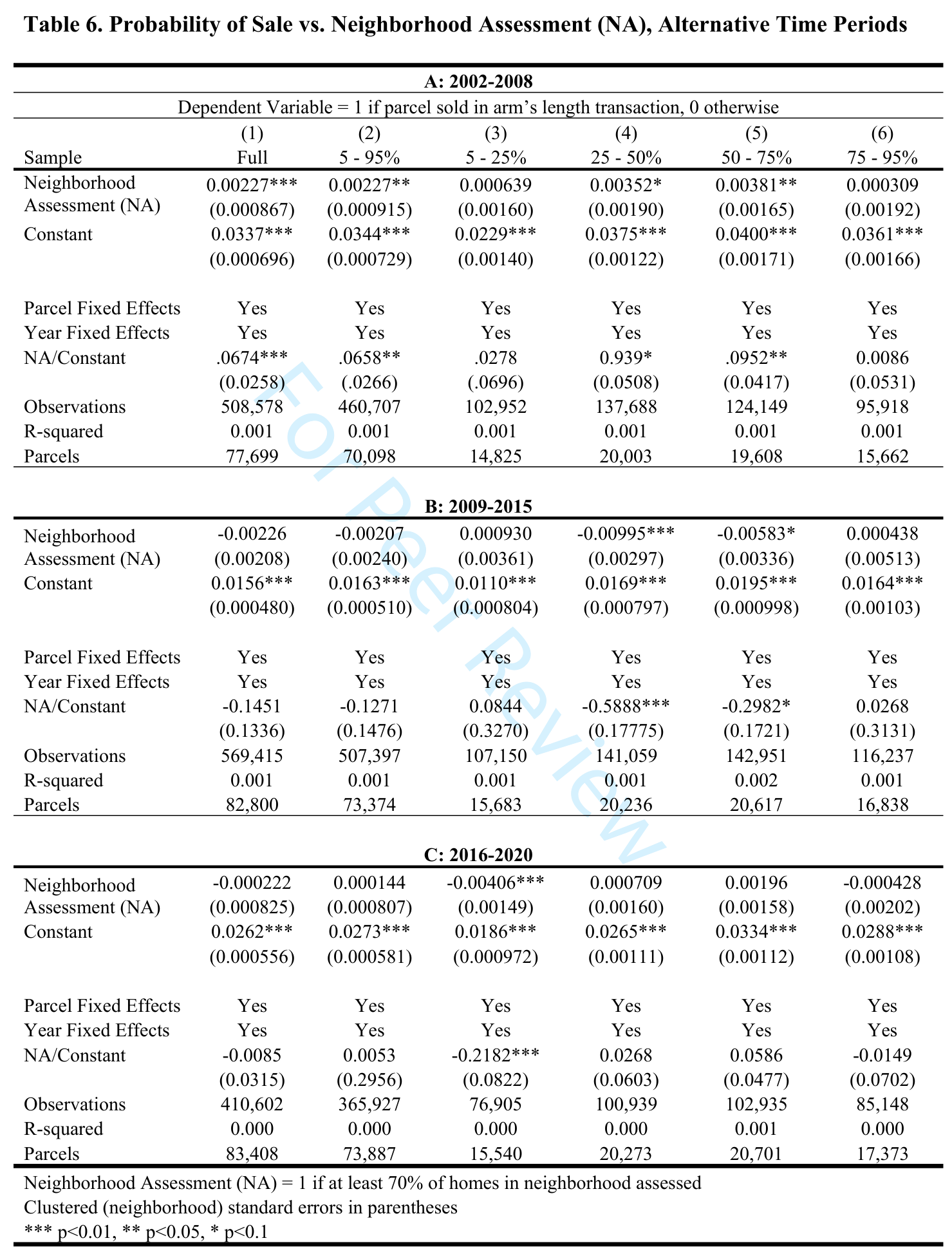### The Effect of Neighborhood Assessments in Different Periods As is clear from Figure 6, the changes in both housing prices and assessed values varied dramatically over this period. Reflecting these differences in both appreciation in prices and assessed values over the period, in Table 6 we report estimates of (5) for three distinct time periods: 2002 – 2008, 2009 – 2015, and 2016 - 2020. For the years 2002 – 2008, the neighborhood assessment had a statistically significant effect on sales for the full sample and for the second and third quartiles. Looking at the row NA/Constant, we see that for these two quartiles, the probability of sale increased by almost ten percent when a neighborhood assessment occurred. A very different story emerges during the 2009 – 2015 period. In this case, the coefficient on the neighborhood assessment in the second and third quantiles are negative – the probability of a sale is reduced with neighborhood assessment. While seeming inconsistent with our results for the samples from 2002 – 2008 and for all years, assessed values decreased from 2011 to 2014, reducing the incentive to sell. Finally, from 2016 – 2020 the only statistically-significant coefficient on neighborhood assessment is for the second quartile and it is negative. 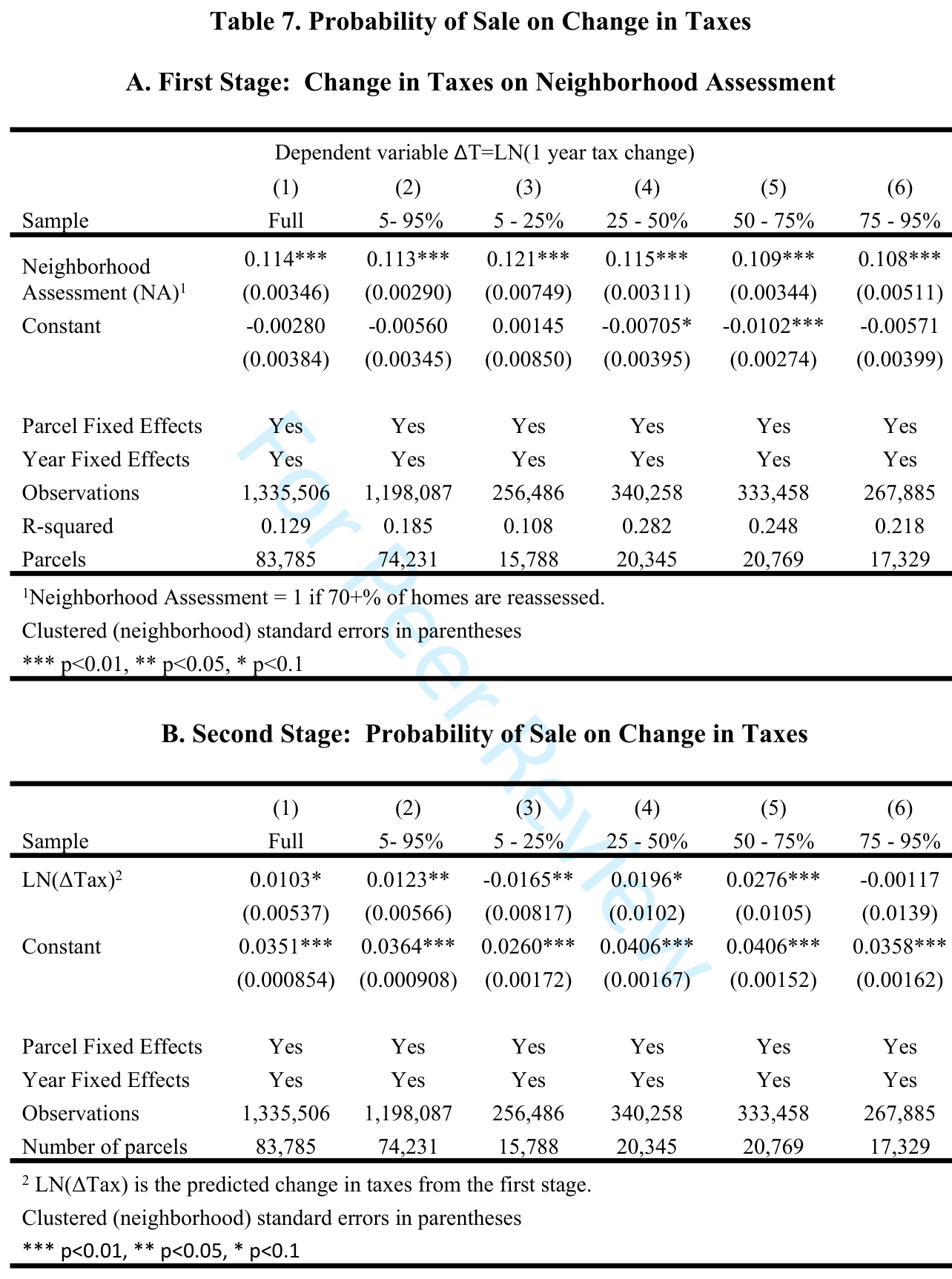### Tax Payments and the Probability of Sale In Table 7 we report our estimate of (6), the relationship between the change in taxes with reassessment and the probability of a sale. In Table 7.A, we report the first stage results, an estimate of the relationship between neighborhood assessment in year _t_ and the (log) tax change from year _t-1_ to year _t_. As seen in the table, a neighborhood assessment increases taxes by approximately 11 percent. Then, using the predicted value for

L N (Δ T)

in the second stage (Table 7B), we estimate the relationship of

L N (Δ T)

with the probability of a sale. The results are qualitatively consistent with the results we found for the relationship between having a neighborhood assessments and the probability of a sale – an increase in the tax payment increases the likelihood of a sale in the full sample and in all but the first and fourth quartile. Interpreting the coefficient on the tax change by dividing by the constant suggests that a ten percent increase in the tax payment increases the probability of a sale by approximately three percent and for the second and third quartiles increases it by 4.8 and 6.8 percent respectively. 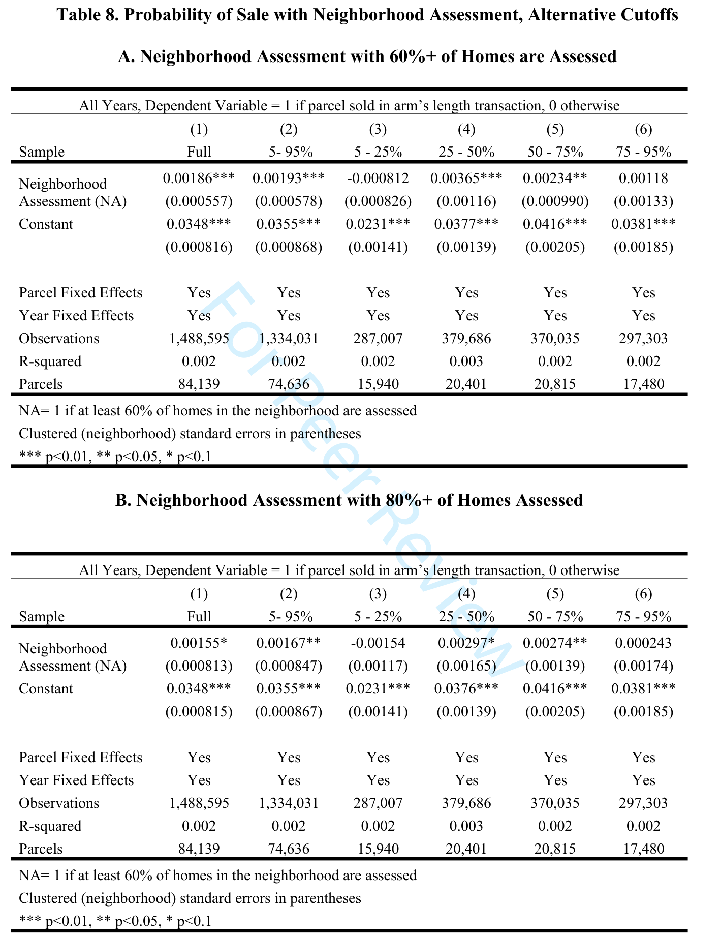### Robustness Checks We undertake several robustness checks reported in Tables 8 – 10. First, we consider alternative cutoffs, in terms of percentage of homes assessed in a neighborhood for the neighborhood to be considered as assessed. We report the results for two alternatives: a neighborhood assessment occurring when 60 percent or more homes are assessed or when 80 percent or more are assessed. Results for a sample of all years (2002–2020) are reported in Table 8. As can be seen by comparing the results in the table to those in Table 5, the coefficients are generally similar in magnitude and statistical significance. 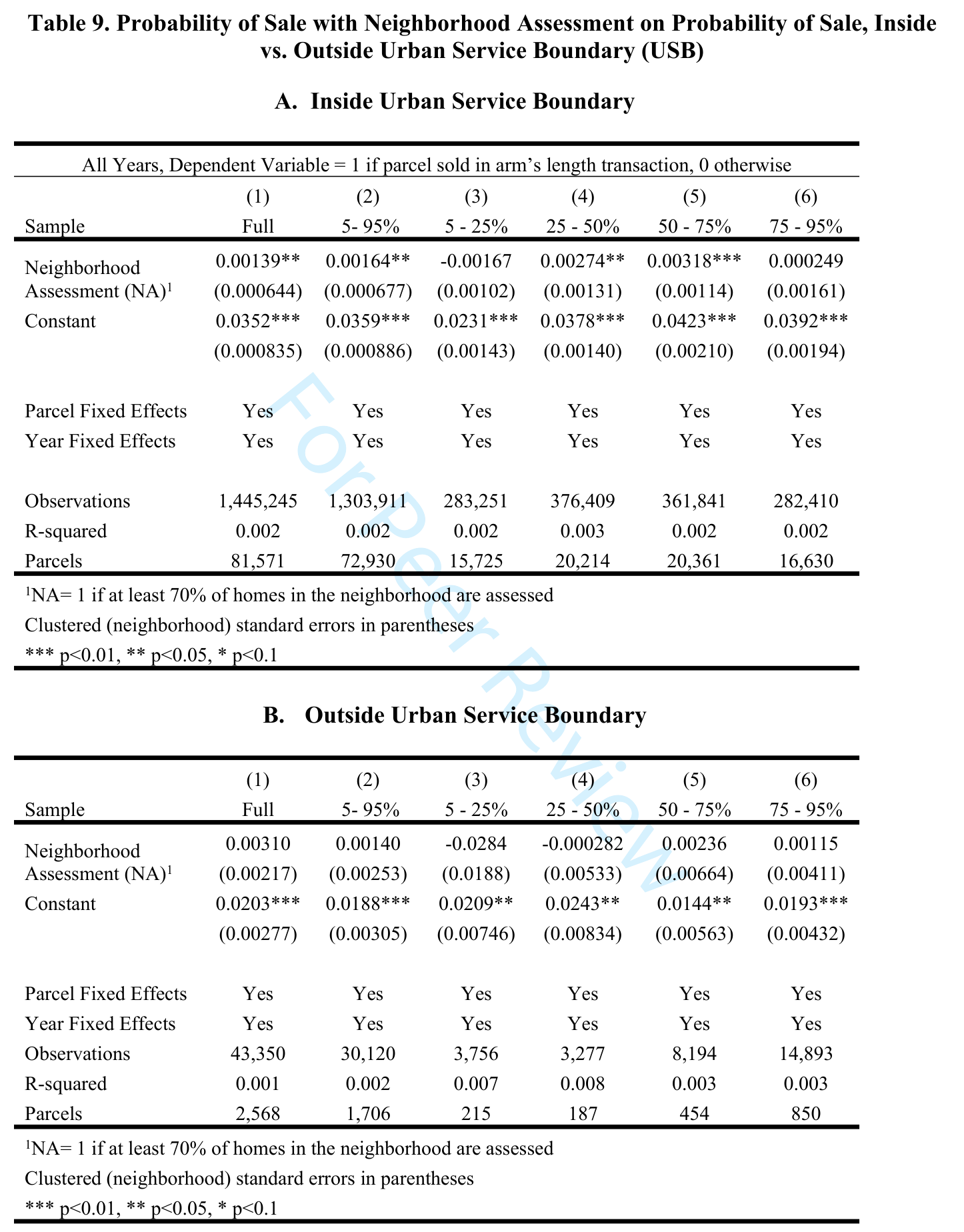Our next robustness check was examining how changes in the sample, specifically dividing the sample based on whether neighborhoods and homes were in or out of the urban service boundary (USB), affected our results. The results in Table 9.A, for the sample in the USB, are almost identical to those for the entire sample reported in Table 5.A. In contrast, the coefficients on neighborhood assessment are not statistically significant for the sample outside of the USB where neighborhoods are newer and more of the housing is associated with agricultural enterprises. 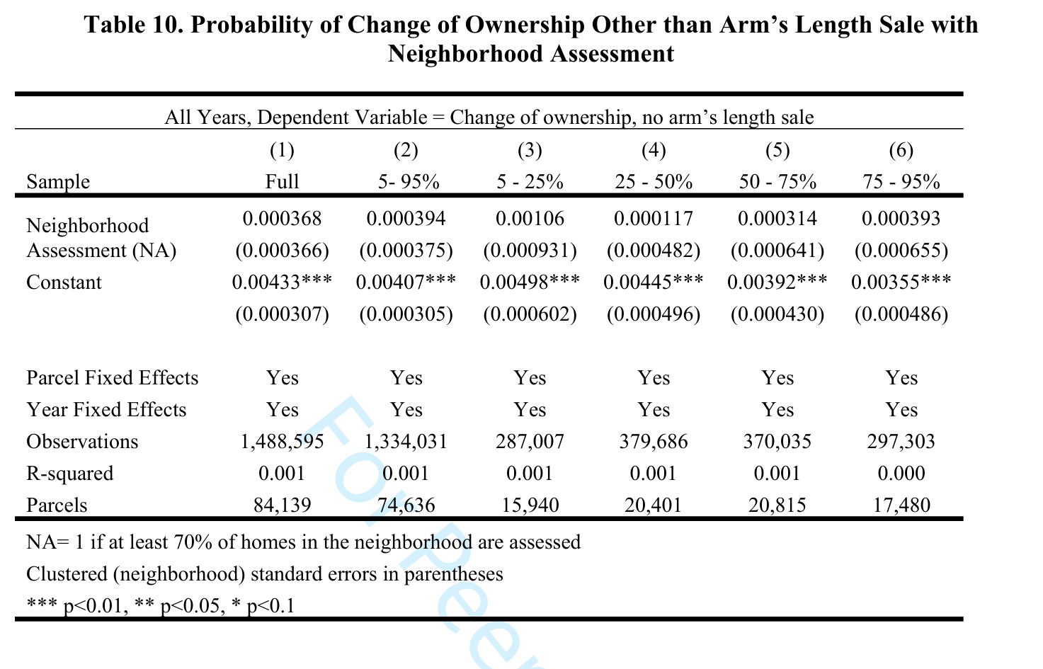Finally, rather than examining the relationship between neighborhood assessments and sales, we examine the relationship of neighborhood assessments with other changes in ownership. These changes often include changes in family status such as marriage, divorce or death of an owner among other reasons. The results, reported in Table 10, show no evidence of any relationship between neighborhood assessment and these ownership changes. This would seem to be consistent with what we would expect – the reasons for these changes in ownership are likely to dominate any efforts at tax planning and are often unavoidable. ## CONCLUSION We find that the practice of infrequent assessments in the face of housing price appreciation can lead to significant tax differentials between properties that have not been reassessed recently and those that have recently been reassessed or sold. Reassessment can result in increases of several hundred dollars per annum in property tax payments. Then, consistent with our expectations, we find that the practice of infrequent neighborhood assessments or upon sales appear to affect household mobility with statistically significant increases in mobility in the year a home is reassessed. Or, as an alternative interpretation, the practice of infrequent assessments reduces mobility in those years when current owners are not facing a neighborhood assessment, thereby receiving a tax advantage relative to purchasers of their properties. Our results suggest that mobility, measured as the sale of a property, is significantly different in the year in which a neighborhood assessment occurs. While these results suggest that mobility is affected by discrete, automatic assessments, it is not obvious as to whether it leads to households postponing moving to capture another year of lower tax obligations or deciding to move earlier to avoid the higher tax payment because of the assessment. Theoretically, both cases are possible. Regardless, while long term mobility might be unaffected by the length of the interval between assessments, our evidence suggests short term mobility rates are affected. To the extent infrequent assessments result in differences in tax liabilities for existing and new owners that influence who lives in a home, there may be “mismatch” in who is residing in the home. This mismatch, arising because decisions about where to live are not determined by households’ valuations of the home independent of their tax obligations, carries an associated welfare cost. ## ACKNOWLEDGEMENTS We thank and wish to acknowledge the helpful comments and suggestions of David Agrawal, Thiess Buettner, Chris Bollinger, Denvil Duncan, John Foster, Christopher Goodman, Raphael Parchett, Louis Warren, Caroline Weber, and seminar participants at the Association of Budgeting and Financial Management (ABFM), the Kentucky Economics Association, the National Tax Association, the University of Kentucky, Universitá sella Svizzera Italiana (Lugano), and FAU Erlangen-Nűrnberg. ## REFERENCES - Anderson, Nathan B. 2006. “Property Tax Limitations: An Interpretative Review”, _National Tax Journal_, 49(3): 685-694. - Bacon-Goodman, Andrew. 2021. “Difference-in-Differences with Variation in Treatment Timing.” _Journal of Econometrics_. 225(2): 254 - 277. - Bowman, John H. 2006. “Property Tax Policy Responses to Rapidly Rising Home Values: District of Columbia, Maryland, and Virginia.” _National Tax Journal_. 59(3): 717-733. - Bradbury, Katharine L., Christopher J. Mayer, and Karl E. Case. 2001. “Property Tax Limits, Local Fiscal Behavior, and Property Values: Evidence from Massachusetts under Proposition 21/2.” _Journal of Public Economics_. 80(2):287-311. - Cabral, Marika and Caroline Hoxby. 2015. “The Hated Property Tax: Salience, Tax Rates, and Tax Revolts.” NBER Working Paper No. 18514. National Bureau of Economic Research, Cambridge, MA. - Cornia, Gary C. and Lawrence C. Walters. 2006. “Full Disclosure: Controlling Property Tax Increases During Periods of Increasing Housing Values.” _National Tax Journal_. 49(3): 735-749. - Chaisemartin, Clement De and Xavier D’Haultfoeuille. 2020. “Two-Way Fixed Effects Estimators with Heterogeneous Treatment Effects.” _American Economic Review_. 111(0: 2964 - 2996. - Chan, S. 2001. “Spatial Lock-in: Do Falling House Prices Constrain Residential Mobility?” _Journal of Urban Economics_. 49(3): 567-586. - Cutler, David M., Douglas W. Elmendorf, and Richard Zeckhauser. 1999. “Restraining the Leviathan: Property Tax Limitation in Massachusetts.” _Journal of Public Economics_. 71(3): 313-334. - Dye, Richard F. Dye, Daniel P. McMillen, and David F. Merriman. 2006. “Illinois's Response to Rising Residential Property Values: An Assessment Growth Cap in Cook County.” _National Tax Journal_, 59(3): 707-716. - Eerola, Essi, Oskari Harjunen, Teemu Lyytikäinen, and Tuuka Saarima. 2021. “Revisiting the effects of housing transfer taxes.” _Journal of Urban Economics_. 124. - Ferreira, Fernando V. 2010. “You Can Take it with You: Proposition 13 Tax Benefits, Residential Mobility, and Willingness to Pay for Housing Amenities.” _Journal of Public Economics_. 94(9-10): 661-673. - Ferreira, Fernando V., Joseph A. Gyourko, and Joseph Tracy. 2010. “Housing busts and household mobility.” _Journal of Urban Economics_. 68(1): 34-45. - Fonseca, Julia and Lu Liu. 2023. “Mortgage Lock-In, Mobility, and Labor Reallocation.” SSRN Working Paper. - Fritzsche, Carolin and Lars Vandrei. 2019. “The German real estate transfer tax: Evidence for single-family home transactions.” _Regional Science and Urban Economics_. 74(1):131-143. - Hodge, Timothy R., Gary Sands, and Mark Skidmore. 2015. “Assessment Growth Limits and Mobility: Evidence from Home Sale Data in Detroit, Michigan.” _National Tax Journal_. 68(3): 573-600. - Hodge, Timothy R., Mark Skidmore, Gary Sands, and Daniel P. McMillen. 2015. “Tax Base Erosion and Inequity from Michigan's Assessment Growth Limit: The Case of Detroit.” _Public Finance Review_. 43(5): 636-660. - Hoyt, William H., Paul A. Coomes, and Amelia S. Biehl. 2011. “Tax Limits and Housing Markets: Some Evidence at the State Level.” _Real Estate Economics_. 39(1): 97-132. - Ihlandfeldt, Keith R. 2011. “Do Caps on Increases in Assessed Values Create a Lock-In Effect? Evidence from Florida's Amendment One.” _National Tax Journal_. 64(1): 7-26. - Lang, Kevin and Tianlun Jun. 2004. “Property Taxes and Property Values: Evidence from Proposition 2 ½.” _Journal of Urban Economics_. 55(3): 439-457. - Nagy, John. 1997. “Did Proposition 13 affect the Mobility of California Homeowners?.” _Public Finance Review_. 25(1): 102-116. - Nakagami, Yasuhiro and Alfredo M. Pereira. 1991. “Housing Appreciation, Mortgage Interest Rates, and Homeowner Mobility.” _Journal of Urban Economics_. 30:271-292. - Quigley, John M. 1987. “Interest Rate Variations, Mortgage Prepayments and Household Mobility.” _The Review of Economics and Statistics_. 69(4): 636. - Shan, Hui. 2010. “Property Taxes and the Elderly.” _Journal of Urban Economics_ 67(2): 194-205. - Skidmore, Mark, Charles L. Ballard, and Timothy R. Hodge: “Property Value Assessment Growth Limits and Redistribution of Property Tax Payments: Evidence from Michigan.” _National Tax Journal_, 63(3): 509-538. - Slemrod, Joel, Caroline Weber, and Hui Shan. 2017. “The behavioral response to housing transfer taxes: evidence from a notched change in D.C. policy.” _Journal of Urban Economics_. 100: 137-153. - Spreen, Thomas Luke and Colton Keddington. 2023. “Temporary Property Tax Relief and Residential Home Sales.” _National Tax Journal_. 76(3): 594-620. - Stansel, Dean B., Gary Jackson, and J. Howard Finch. 2007. “Housing Tenure and Mobility with an Acquisition-Based Property Tax: The Case of Florida.” _Journal of Housing Research_. 16(2): 117-129. - Stohs, Mark Hoven, Paul Childs and Simon Stevenson. 2001. “Tax Policies and Residential Mobility.” _International Real Estate Review_. 4(1): 95-117. - Wasi, Nada, and Michelle J. White. 2005. _Property Tax Limitations and Mobility: Lock-In Effect of California's Proposition 13_. Brookings Institution Press. Washington, DC. - Zhang, Yanjiang and Yonghen Deng. 2023. “Duration-dependent transaction tax effects on sellers and their behaviors.” _Real Estate Economics_. (online version: https://onlinelibrary.wiley.com/doi/10.1111/1540-6229.12441 ### Figure 1 Annual and Present Value Differences in Taxes during Assessment Cycle, Current Versus New Owner for Different House Values (% of Distribution)

Figure 1 has two bar-chart panels comparing current-owner and new-owner taxes over a three-year assessment cycle for houses at four sale-price percentiles. Annual tax differences rise by year; present-value differences peak in the second year. Full assumptions and house-value note appear. — Figure 1. Open full-resolution image.

### Figure 2 Assessment Appreciation and Tax Payments: Assessment Limit versus Periodic Assessment Limit vs. Neighborhood Reassessment (Full & Partial) versus Market Value

Figure 2 compares annual property-tax payments over sixteen years under market-value taxation, an assessment limit, and full or partial neighborhood reassessment. Market-value payments rise steadily while reassessment schedules rise in steps; the printed source assumptions remain. — Figure 2. Open full-resolution image.

### Figure 3 Map of House Sales in Fayette County, 2002 – 2020

Figure 3 maps house sales in Fayette County from 2002–2020. Individual sale points cluster densely in the central and southwestern developed areas, with fewer points in the rural northern and southeastern areas. — Figure 3. Open full-resolution image.

### Figure 4A Lexington Housing Price Index (FHFA) and Urban CPI, (semi-annual) 2002 – 2020 (relative to 1-2002)

Figure 4A compares Lexington’s house-price index with urban CPI from 2002–2020, normalized to early 2002. House prices flatten around 2009–2014, then rise faster than CPI through 2020; the source attribution remains. — Figure 4A. Open full-resolution image.

### Figure 4B 30-Year Fixed Rate Mortgage Average in United States, November 2001 – January 2021

Figure 4B plots the U.S. average thirty-year fixed mortgage rate from November 2001 to January 2021. Rates fluctuate while declining from about seven percent to below three percent, with dates and FRED source attribution. — Figure 4B. Open full-resolution image.

### Figure 5 Neighborhood Assessment Timing and Tax Payments ($2020), 2002 – 2020

Figure 5 plots mean and house-value-quartile tax payments around neighborhood reassessment. Payments rise at reassessment year zero in each group, with the largest dollar increase in the highest quartile; source definitions remain. — Figure 5. Open full-resolution image.

### Figure 6 Mean Sale Price vs. Mean Assessment, 2002 – 2020

Figure 6 compares mean sale prices with mean assessed fair cash values in 2020 dollars from 2002–2020. Sale prices generally exceed assessments, with the gap widening markedly after 2014. — Figure 6. Open full-resolution image.

### Figure 7 Change in Tax Payment from Sale vs. Non-Sale with Neighbor Assessment, by Assessment Quartile, 2002–2020

Figure 7 compares changes in tax payments after sales with changes under neighborhood reassessment, overall and by assessment quartile. Sales show the larger change in every displayed group; the full neighborhood-assessment definition accompanies the chart. — Figure 7. Open full-resolution image.

### Figure 8 Estimated Change in Probability of Sale (%) with Neighborhood Assessment

Figure 8 has two panels of estimated percentage changes in sale probability: by assessment-value quantile and by the share of neighborhood homes assessed. It includes significance markers, reassessment definition, category labels and the full color legend. — Figure 8. Open full-resolution image.

### Figure A1 Neighborhood Assessment Timing and Tax Payments ($2020), Various Periods

Figure A1 plots mean and quartile tax payments around reassessment in three periods: 2002–2008, 2009–2015 and 2016–2020. Each panel retains its period title, axes, quartile labels and source-definition note. — Figure A1. Open full-resolution image.

### Figure A2 Change in Tax Payment from Sale vs. Non-Sale with Neighbor Assessment, by Assessment Quartile, Various Periods

Figure A2 compares tax-payment changes after sales and neighborhood reassessments by assessment quartile in three periods. Paired colored bars, the period titles and the complete authors’ definition note are visible. — Figure A2. Open full-resolution image.

### Table 1 State Laws Governing Frequency of Real Property Assessment

Table 1 lists state laws governing real-property reassessment frequency, arranged in two state-and-frequency column pairs. It includes all state entries, cited sources and five state-specific footnotes. — Table 1. Open full-resolution image.

### Table 2 Neighborhood Assessment Rates, 2003 – 2020 (Percentage of Homes Assessed)

Table 2 lists annual percentages of homes assessed in named Fayette County neighborhoods from 2003–2020. Highlighted cells mark large reassessment episodes; all neighborhood rows and year columns are visible. — Table 2. Open full-resolution image.

### Table 3 Summary Statistics on Sales, Value, and Length of Ownership

Table 3 summarizes sales, assessed values and ownership duration for the full sample and assessed-value quantiles. It includes sale timing around reassessment, parcel and observation counts and the distribution-definition footnote. — Table 3. Open full-resolution image.

### Table 4 Assessed (Fair Cash) Value and Neighborhood Assessment

Table 4 estimates log assessed fair-cash value for six value-based samples. Neighborhood assessment, house-price index, assessment timing and tenure coefficients appear with fixed-effect indicators, sample statistics and full notes. — Table 4. Open full-resolution image.

### Table 5 Probability of Sale vs. Neighborhood Assessment

Table 5 estimates sale probability by neighborhood reassessment for six assessed-value samples. Panel A uses a reassessment indicator and Panel B separates four reassessed-share ranges; coefficients, fixed effects, sample statistics and notes are complete. — Table 5. Open full-resolution image.

### Table 6 Probability of Sale vs. Neighborhood Assessment (NA), Alternative Time Periods

Table 6 repeats sale-probability estimates for 2002–2008, 2009–2015 and 2016–2020. Each period has six value-based samples, coefficients, fixed-effect indicators, relative effects and observation counts, followed by full model notes. — Table 6. Open full-resolution image.

### Table 7 Probability of Sale on Change in Taxes

Table 7 has a first-stage model of tax changes on neighborhood reassessment and a second-stage model of sale probability on predicted tax changes. Both six-column panels include uncertainty estimates, fixed effects, sample counts and definitions. — Table 7. Open full-resolution image.

### Table 8 Probability of Sale with Neighborhood Assessment, Alternative Cutoffs

Table 8 tests alternative neighborhood-reassessment cutoffs of sixty and eighty percent. Both six-column panels contain coefficients, fixed effects, sample statistics and source-printed notes. — Table 8. Open full-resolution image.

### Table 9 Probability of Sale with Neighborhood Assessment on Probability of Sale, Inside vs. Outside Urban Service Boundary (USB)

Table 9 estimates sale-probability effects separately inside and outside the urban service boundary, across six value-based samples. Both panels retain standard errors, fixed effects, observation counts and the reassessment definition. — Table 9. Open full-resolution image.

### Table 10 Probability of Change of Ownership Other than Arm’s Length Sale with Neighborhood Assessment

Table 10 estimates changes of ownership other than arm’s-length sales in relation to neighborhood reassessment. Six value-based samples show coefficients, fixed effects, sample statistics and complete notes. — Table 10. Open full-resolution image.

### Table A1 Differences in Present Value of Taxes, Current vs. New Owner by Years Since Assessment

Table A1 lays out current-owner and new-owner tax payments by years since assessment and sale year, then present-value tax differences. The full symbolic expressions, general formula and printed variable-definition note are retained. — Table A1. Open full-resolution image.

### Table A2 Summary Statistics on Housing Characteristics

Table A2 summarizes housing size, age, construction, amenities and room counts for the full sample and assessed-value quantiles. Parcel, year and observation counts and the distribution-definition footnote appear. — Table A2. Open full-resolution image.

### Table A3 Estimation of P(Sales) with Heterogeneous Treatment Effects

Table A3 estimates heterogeneous neighborhood-assessment effects on sale probability for all years and three subperiods. Each six-column panel includes coefficients and observations, followed by clustered-error, method and treatment-definition notes. — Table A3. Open full-resolution image.

--- ## Notes

1. That assessments might seem subjective to the taxpayer is perhaps reflected in the increasing numbers of homeowners appealing property tax assessments (Forbes (June 8, 2011)).

2. While the late 1970’s and early 1980’s was a period in which several states imposed or revised property tax limits, in fact, Missouri first instituted rate limits on property taxes in 1875. States without any state limits on property taxes include Connecticut, Hawaii, Maine, New Hampshire, South Carolina, Vermont, and Virginia. The District of Columbia has no restrictions on property taxes as well. See Hoyt, Coomes, and Biehl (2011) for more detail on the form and timing of state property tax limits.

3. From the Kentucky Revised Statute 132.690 Annual revaluation of real property – Quadrennial physical examination of real property – Methods of examination – Emergency revaluation. (1) (a) Each parcel of taxable real property or interest therein subject to assessment by the property valuation administrator shall be revalued during each year of each term of office by the property valuation administrator at its fair cash value in accordance with standards and procedures prescribed by the department and shall be examined no less than once every four (4) years by the property valuation administrator.

4. See the discussion in Fereira (2010).

5. For example, real housing appreciation in San Francisco has exceed the national average by more than 2 percentage points per year for the years between 1950 and 2000 (Gyourko 2013).

6. As we only consider arms-length sales of owner-occupied houses, a sale of a property results in a change in residence for both the seller and purchaser of the property.

7. The Federal Housing Finance Agency (FHFA) housing price index (HPI) for the Lexington MSA increased by 2.82 percent from 2002 to 2020.

8. As seen in the formulae in Appendix Table A1, critical to the tax savings received by an existing homeowner is the rate of appreciation in housing prices, the value of the home, the tax rate, and the length of time until the next assessment.

9. In the case of an uncertain reassessment, the expect present value of tax savings for a current owner is given by $E P V \equiv \sum_{t = 0}^{\overset{―}{T}} P (N A (t)) p V^{0} \sum_{k = 0}^{t - 1} \frac{(1 + ρ)^{k} - 1}{(1 + r)^{k}}$ where $P (N A (t))$ is the probability of a neighborhood reassessment in year $t$ , $p$ is the tax rate, $V^{0}$ is the initial assessment, $ρ$ is the appreciation rate, $r$ is the discount rate, with a reassessment to occur sometime before or at $t = \overset{―}{T}$ .

10. From the Fayette County PVA website (https://fayettepva.com/assessments-appeals/): “Many homeowners will receive an assessment notice that will include a map of recent sales in their immediate neighborhood in April. Neighborhood sales are the primary driver for reassessments.” Thus current homeowners will be informed of their (re)assessed value by April of the year of reassessment.

11. We have obtained data from the Fayette PVA from 2004 onward that shows us which neighborhoods were subject to assessment, allowing us to explore the effects of binding versus non-binding assessments more carefully.

12. As robustness checks, we considered 60% and 80% as alternative criteria for binding assessments.

13. Shan (2010) finds smaller OLS estimates than IV estimates due to omitted variable bias.

14. For houses that were in the sample in 2002, there assessed value (in $2020) would depend in which quartile they belong. Regardless of changes in how their relative value might change over time they remain in the same quartile. Houses that enter the sample later are categorized based on how they rank relative to the houses in 2002 based on their $2020 value.