# Real estate agent dynamism and licensing entry barriers
**Authors:** Samuel J. Ingram and Aaron Yelowitz.
**Source edition:** Journal of Entrepreneurship and Public Policy, publisher early-view article. DOI: 10.1108/JEPP-07-2019-0063. © Emerald Publishing Limited.
**Affiliation:** Department of Economics, University of Kentucky, Lexington, Kentucky, USA.
**Article history:** Received 31 July 2019; revised 10 September 2019; accepted 10 September 2019.
**Paper type:** Research paper
## Abstract
Purpose – The purpose of this paper is to examine the labor market entry of real estate agents in the USA and the potential effect of occupational licensing on entry. Design/methodology/approach – Data from the 2012 to 2017 American Community Survey are linked to local housing price fluctuations from the Federal Housing Finance Agency for 100 large metro areas. The cost of entry associated with occupational licensing for new real estate agents is carefully measured for each market and interacted with housing fluctuations to investigate the role for barriers to entry. Findings – A 10 percent increase in housing prices is associated with a 4 percent increase in the number of agents. However, increased license stringency reduces the labor market response by 30 percent. The impact of
licensing is stronger for women and younger workers. Originality/value – This work contributes to the growing literature investigating the impact of occupational licensing on labor supply and entry in the USA, as well as potential impacts of regulation on dynamism and entrepreneurship. To the authors’ knowledge, this study is also the first to quantify the cost of occupational licensing in the real estate industry.
**Keywords:** Female entrepreneurs, Entrepreneurship, Occupational licensing, Real estate agents, Entry barriers
## 1. Introduction
In 2017, the total value of all US homes was $31.8 trillion1, with approximately 4.8m existing homes sold2. There are about 2m active real estate licensees (approximately 1.2 percent of the total labor force), with nearly 1.4m being members of the National Association of Realtors (NAR)®3. The majority of Realtors® do not have a baccalaureate degree and are independent contractors within their firm, highlighting opportunities for entrepreneurship within the industry.
Recent studies have focused on the absence of commission competition (Barwick and Pathak, 2015; Hsieh and Moretti, 2003) even in the presence of substantial entry. Individuals seeking employment in real estate face arguably modest barriers to entry through occupational licensing. In this paper, the analysis explores the degree to which these modest licensing barriers affect an individual’s entry and labor supply in real estate. The ability to identify convincingly the causal effect of occupational licensing is difficult in many contexts, including this setting, because the main source of variation is cross-sectional differences in the stringency of licensing requirements at the state-level. Other factors, such as a state’s overall regulatory environment toward entry-level workers, may conflate the estimated impact of occupational licensing. There
is little temporal variation in licensing requirements within a state for most occupations, so a straightforward “difference-in-differences” methodology afforded in other labor market contexts such as minimum wages cannot be used effectively here (Neumark and Wascher, 2008). To circumvent this difficulty, and control for unobserved, fixed geographic heterogeneity, this paper uses exogenous housing appreciation shocks to local markets to identify the effect of occupational licensing.
To illustrate this approach, consider the localities of Milwaukee, Wisconsin and Columbus, Ohio. These Midwest cities have similar populations and housing prices. The average 2017 price of a single family home was approximately $186,000 in Milwaukee and $182,000 in Columbus. From 2012 to 2017, Milwaukee had a 16 percent increase in home prices while Columbus had a 28 percent increase. If agents enter the market freely and commission rates are fixed, the theoretical prediction would be that Columbus should have had greater agent entry than Milwaukee (Hsieh and Moretti, 2003). In practice, the Columbus market had a 29 percent increase in the number of agents, smaller than Milwaukee’s 64 percent increase, despite having more rapid appreciation.
A key difference that explains the diminished growth is that Ohio is one of the most expensive states to obtain an agent license, while Wisconsin has average costs.
The approach employed here exploits the robust finding in previous research that real estate agents enter the market when housing prices increase (Hsieh and Moretti, 2003). The analysis utilizes housing price fluctuations from the 2012–2017 Federal Housing Finance Agency’s (FHFA) housing price index linked to agent characteristics in local markets (core-based statistical areas or CBSAs) using microdata from the American Community Survey (ACS). Careful measurement of state-level occupational licensing costs for new agents are interacted with local housing price changes using a difference-in-differences design. The results show that a 10 percent increase in housing prices leads to 4 percent more agents. More stringent licensing reduces this labor entry by approximately 30 percent. The results also suggest larger impacts of licensing costs on women and workers
younger than 50.
In addition to providing a more compelling framework for estimating the impact of occupational licensing, this paper makes several other contributions. Using a variety of data sources, the cost barriers to entry in real estate are carefully quantified across states. To the authors’ knowledge, this study is the first to do so in real estate. Such costs include the licensing fee paid to the state, course fees, and the opportunity cost of time from taking the required courses. The cost varies from $0 to $3,506 across states, with a median total cost of $1,697. Overall, the magnitude of such entry costs in real estate from occupational licensing might be considered modest compared with other professions. The results shown below suggest relatively small barriers
may have significant effects, raising the possibility of larger responses in similarly skilled occupations with more costly barriers.
This paper contributes to a growing literature on the impact of licensing on labor supply and entry. Recent work by Blair and Chung (2018) and Kleiner and Soltas (2019) suggests licensing reduces labor supply at the national level, aggregating across all occupations. Other works investigate these issues at the occupation level including massage therapists (Thornton and Timmons, 2013), cosmetologists (Zapletal, 2017), certified public accountants (Stephenson and Meehan, 2018) and dentists (Kleiner and Kudrle, 2000). Kleiner (2006) has a brief overview of the potential labor supply effects of licensing and reviews some previous empirical research. In addition, Cathles et al. (2010) look at the differential effect of licensing costs on the labor supply of men and women by analyzing the barriers to entry for funeral directors and finds that
women are more affected by these policies. These papers suggest that licensing reduces labor supply and may have differential effects on subpopulations.
This paper also contributes to the research investigating the impact of regulation on dynamism and entrepreneurship. Goldschlag and Tabarrok (2018) discuss potential impacts of regulation on dynamism through entry and exit rates. Policy pieces have also highlighted this connection including Mellor and Carpenter (2016), Slivinksi (2015) and Wiens and Jackson (2015). In academic research, with specific focus on occupational licensing, Prantl and Spitz-Oener (2009) investigate the relationship between licensing, self-employment and entry in reunified Germany. They find that licensing requirements reduce entry into self-employment, with stronger effects in labor markets with lower average education levels. In addition, Cebula et al. (2018) note that regulation and licensing have effects on living conditions and the local economy.
The real estate agent labor market is dynamic and entrepreneurial, with more than half of the agents in the ACS sample reporting they are self-employed. Comparing real estate agents to other occupations using the Current Population Survey’s (CPS) Tenure and Mobility Supplement, agents have above average earnings and, after controlling for age, have lower tenure rates than other occupations. Agents are also more likely to work part-time. This is also a noteworthy labor market to analyze entrepreneurship, as there are considerably more female real estate agents than there are male real estate agents.
The combination of a dynamic, entrepreneurial occupation and the geographic variation in both entry costs and entry incentives provide a unique opportunity to investigate the role of regulatory barriers on labor market response. The paper proceeds with Section 2 reviewing the real estate licensing literature. Section 3 presents the estimated cost of real estate licensing by state and reviews the housing and labor market data. Section 4 presents the results and Section 5 concludes.
## 2. Literature review
Vorotnikov (2011) has a brief historical review of real estate licensing. These regulations started as far back as the 1870s and originally contained no requirements to obtain a license, other than paying a fee to the local real estate board. These local boards transformed into the current licensing system as state professional groups advocated for more stringent entry restrictions in the occupation. Vorotnikov highlights the evolution of the NAR® from these local and state professional groups into the primary institution supporting real estate licensing policies. The NAR (2019) currently describes themselves as “America’s largest trade association, representing 1.3 million members.”
A few studies have looked at the impact of occupational licensing on real estate agents. A series of papers in the 1980s investigated agent licensing with data available at the time. Carroll and Gaston (1983) review their previous research, which analyzes licensing pass rates and the number of days houses sit vacant, and find a reduction in the number of agents results in lower service quality. Johnson and Loucks (1986) find that licensing reduces the number of agents in the market but may also decrease the number of complaints. Both Guntermann and Smith (1988) and Shilling and Sirmans (1988) find fewer complaints against agents in areas with high licensing barriers and the latter paper also finds that licensing boards decrease the pass rates on exams
to deter new entry. Powell and Vorotnikov (2012) follow up on this line of questioning by analyzing the real estate market in Massachusetts following an increase in the required continuing education hours. The authors find no decrease in complaints but do find a significant reduction in the number of agents and an increase in earnings.
When determining the scope of agent licensing, a distinction should be made between real estate sales agents and real estate brokers. While this distinction is discussed in the previous academic literature, regulations do not use these terms consistently from one state to the next. NAR (2019) segments these titles by designating agents as the sales force and brokers as the managers. Most states have separate licenses for brokers that are more stringent than agent licenses. The classification of sales agent licensing used in this paper is taken from the published national databases described below. In these national data sets, five states are excluded from having specific agent licenses (Colorado, Oregon, Illinois, Indiana and North Carolina). The real estate regulatory environment in
these states differs from the other 46 jurisdictions. Specifications are conducted with and without these states and qualitatively similar results are found.
## 3. Data and methodology
### 3.1 Estimated total licensing costs
This section estimates the licensing entry cost for new agents for each state as well as the District of Columbia (DC) and gives an overview of the housing data4. The data for the licensing calculations are collected from various sources including the 2011–2017 CPS (Flood et al., 2018), the National Council of State Legislature’s National Occupational Licensing Database (NCSL, 2019), The Knee Center for the Study of Occupational Regulation’s National Database (CSOR, 2019), state regulatory websites and various state education provider websites. More details on the information collected from these sources, the methods of collection and the calculations used for analysis are described below.
The cost of entry associated with licensing is calculated from the licensing fees for each state, the cost of educational training courses required by the state, the hours of training required and the average opportunity cost of training in each state, s:
**Equation (1):**
**Equation (1)**
Figure 1 shows the 2019 variation in total licensing cost by state and Table I provides the licensing requirements and component costs for each state. The median entry cost is $1,697.
Three states (Texas, South Dakota and Ohio) have estimated entry costs of more than $3,000. These states all require more than 100 h of training (along with Utah and California).
Also, note that in Ohio and South Dakota the average required coursework costs more than $1,000. This is compared to an average course cost in other states of $345. Table II shows that the variation in entry cost does not appear to be driven by region but occurs within region. Following the procedures described below, Oregon, Colorado, Illinois, Indiana and North Carolina are designated with no entry costs for new agent licenses. These states are listed as unlicensed for agents in both the NCSL and the CSOR databases. As discussed above, these states may have licensing requirements for brokerage activity and the primary analysis is robust to excluding these states.
### 3.2 Licensing fees by state
Each state typically requires applicants to pay a fee after the completion of coursework and exams. The state then reviews the application and confirms the applicant as a licensed real estate agent.
The licensing fee information is primarily collected from the CSOR and NCSL databases. The fee estimates from the two sources are similar but have meaningful differences.
### Figure 1. Total licensing entry cost by state
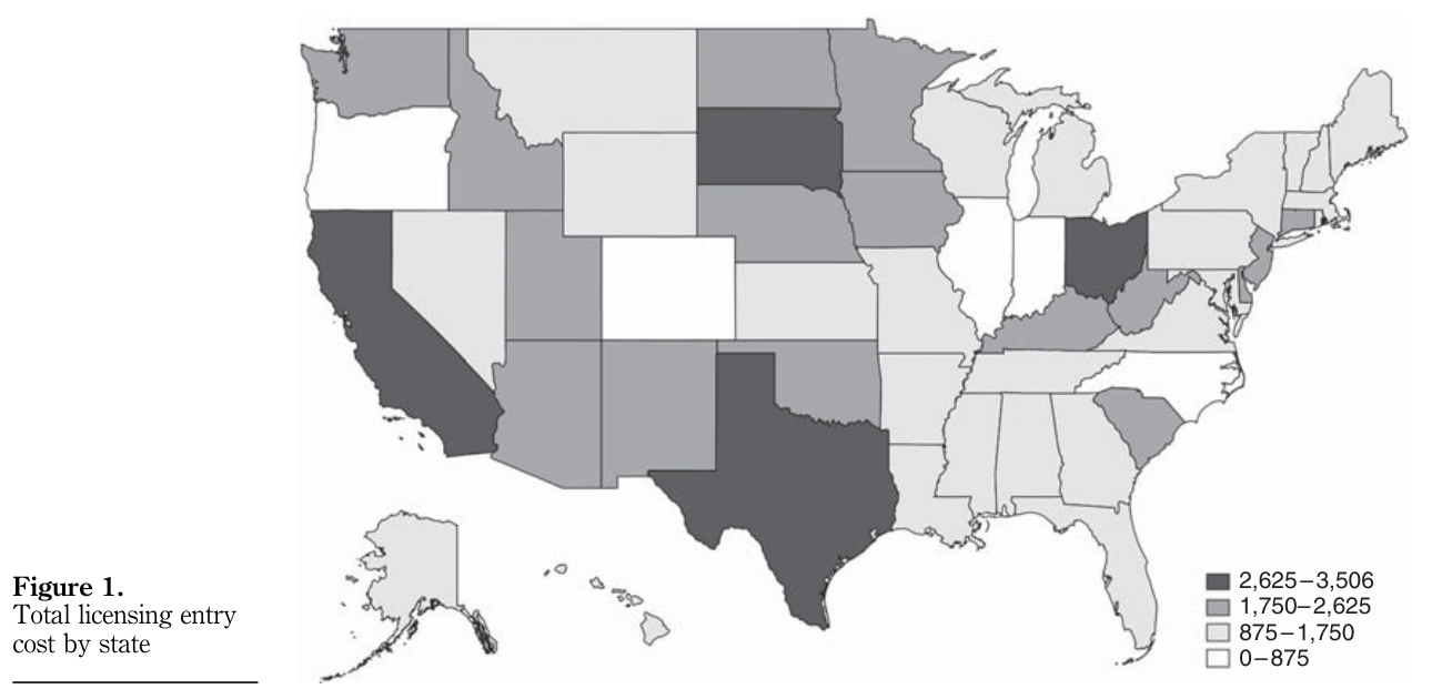 Figure 1. Open full-resolution image.
**Caption:** Total licensing entry cost by state.
There are several reasons for differences in these measures. First, the timing of the data collection may have differed. Additionally, a goal of both databases is to make licensing information more transparent and comparable across occupations. This may lead to slight variations in order to make these estimates more generalizable to multiple occupations.
### Table I. Real estate licensing summary by state
Figure 1. Open full-resolution image.
**Caption:** Total licensing entry cost by state.
There are several reasons for differences in these measures. First, the timing of the data collection may have differed. Additionally, a goal of both databases is to make licensing information more transparent and comparable across occupations. This may lead to slight variations in order to make these estimates more generalizable to multiple occupations.
### Table I. Real estate licensing summary by state
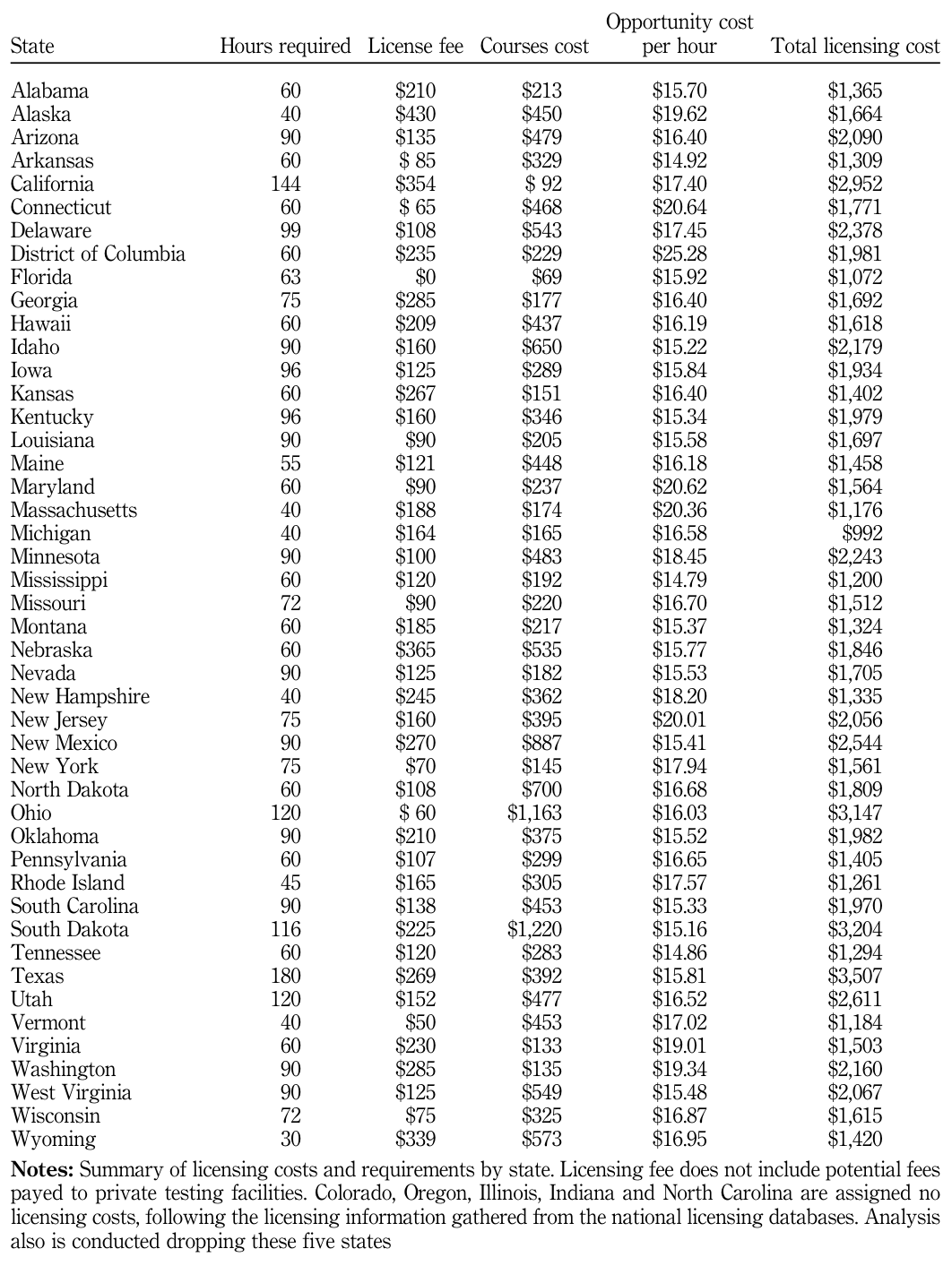 Table I. Open full-resolution image.
### Table II. Total licensing entry cost by region
Table I. Open full-resolution image.
### Table II. Total licensing entry cost by region
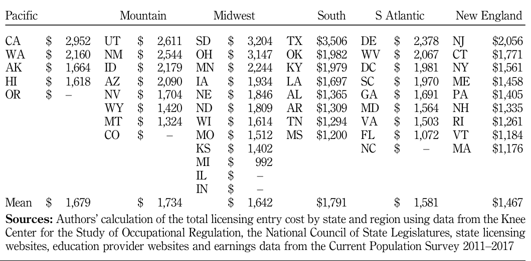 Table II. Open full-resolution image.
From the follow-up procedure used here, discrepancies are less likely caused by errors in the data gathering process and more likely reflect opaqueness of the licensing policies. Although there are small differences in the database estimates of the fees by state, it is preferred to use a preexisting measure when available. The correlation for the fees in the two databases is 0.67. These fees were then verified manually to confirm their accuracy. To obtain the final licensing fee, this paper used the following procedure: first, if the licensing rates were within $100, the lower of the two fees were used and the state website was inspected to confirm the fee. (In 20 of the states the fees were either identical or within $10 and 43
states had fees listed in the two databases within $100, with a median difference of $15). Second, for the last nine states, the state websites were inspected and compared with the values provided in the databases. The current fee listed on the website was used and the website links were recorded. The final licensing fee estimates have a correlation of 0.86 with the CSOR database and 0.84 with the NCSL database.
The fees vary considerably by state, from $0 to $430 (Alaska). A total of 16 states have fees over $200 and 20 states have fees between $100 and $200. Ten states have fees less than $100. The median fee is $135.
### 3.3 Cost of training courses
The required course training is typically conducted by a state approved instructor or education facility. These education providers must obtain a separate license for instruction. The cost of these required training courses was not readily available in either national database.
The coursework is offered at a fixed cost and typically includes all required course material to meet the licensing requirements. To obtain an estimate of the training cost by state a combination of national and local prices were used. Three large online providers offered courses for a variety of states. Site 1 offered 22 states, Site 2 offered 11 states and Site 3 offered 25 states. Two additional prices were estimated for every state after searching for local providers. The type of provider varied and included community colleges, university campuses, individual agents conducting seminars or workshops and private education training centers.
The 150 prices gathered provide a minimum of 2 and a maximum of 5 prices for each state. The two lowest prices are averaged to obtain an estimate of the cost of training in each state. This information is included in Table III. The median course cost is $338. South Dakota and Ohio have the most expensive training courses at $1200 and $1163, respectively.
### Table III. Pre-licensing course cost by state
Table II. Open full-resolution image.
From the follow-up procedure used here, discrepancies are less likely caused by errors in the data gathering process and more likely reflect opaqueness of the licensing policies. Although there are small differences in the database estimates of the fees by state, it is preferred to use a preexisting measure when available. The correlation for the fees in the two databases is 0.67. These fees were then verified manually to confirm their accuracy. To obtain the final licensing fee, this paper used the following procedure: first, if the licensing rates were within $100, the lower of the two fees were used and the state website was inspected to confirm the fee. (In 20 of the states the fees were either identical or within $10 and 43
states had fees listed in the two databases within $100, with a median difference of $15). Second, for the last nine states, the state websites were inspected and compared with the values provided in the databases. The current fee listed on the website was used and the website links were recorded. The final licensing fee estimates have a correlation of 0.86 with the CSOR database and 0.84 with the NCSL database.
The fees vary considerably by state, from $0 to $430 (Alaska). A total of 16 states have fees over $200 and 20 states have fees between $100 and $200. Ten states have fees less than $100. The median fee is $135.
### 3.3 Cost of training courses
The required course training is typically conducted by a state approved instructor or education facility. These education providers must obtain a separate license for instruction. The cost of these required training courses was not readily available in either national database.
The coursework is offered at a fixed cost and typically includes all required course material to meet the licensing requirements. To obtain an estimate of the training cost by state a combination of national and local prices were used. Three large online providers offered courses for a variety of states. Site 1 offered 22 states, Site 2 offered 11 states and Site 3 offered 25 states. Two additional prices were estimated for every state after searching for local providers. The type of provider varied and included community colleges, university campuses, individual agents conducting seminars or workshops and private education training centers.
The 150 prices gathered provide a minimum of 2 and a maximum of 5 prices for each state. The two lowest prices are averaged to obtain an estimate of the cost of training in each state. This information is included in Table III. The median course cost is $338. South Dakota and Ohio have the most expensive training courses at $1200 and $1163, respectively.
### Table III. Pre-licensing course cost by state
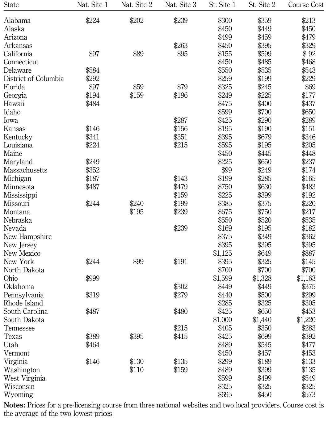 Table III. Open full-resolution image.
Table III reveals there is considerable heterogeneity in price across states. The prices are also competitive within a state, even across different types of providers (such as online versus in-person instruction). Note, for example, Alabama and Hawaii, both offer 60 h courses and both have online and in-person course options. The national sites offer competing rates in Alabama of $224, $202 and $239. For an online course with the same number of hours in Hawaii, the national provider charges $484 and the two local providers charge $475 and $400, respectively. Another example is North Dakota, which does not have a course listed with the national providers but the two local options both charge a price of $700. Another interesting example is California ($92) and Florida ($62), which have some of the strictest hours requirements but lowest course prices, potentially because of more competition among education providers in these states along with a larger population of agents, decreasing the marginal cost.
### 3.4 Required training hours by state
States with explicit licensing entry restrictions require a certain number of hours of state approved real estate education. The requirements were first gathered from the NCSL and CSOR databases and then verified on each state’s website. A total of 33 of the states’ training hours requirements were identical in both the NCSL and the CSOR databases. For any differences in these databases, the hours requirement was either verified or a new hours requirement was found on the state’s licensing website.
There is large variation in the required hours of training for each state as shown in Figure 2. The required hours of education training vary from 30 h in Wyoming to 180 h in Texas. The median hours requirement for states that have an initial sales license is 68 h. A total of 18 states require 90 h or more and 7 states require less than 50 h.
One limitation in many licensing studies is the cross-sectional nature of licensing policies and the lack of variation over time. This study circumvents this problem by assuming relatively constant licensing costs and utilizing labor demand shocks to identify the licensing effect. To verify consistency of the licensing policies over time, archived licensing websites were used to investigate the 2012 licensing requirements. The hours requirements changed in two states over the sample period. California increased the required hours of training, while Texas decreased the hours requirement in 2012, the first year of the sample. (In addition, the licensing fees differed by $24 and had a correlation of 0.84 with the current licensing fees.) This suggests that licensing requirements and costs may be relatively stable over
this six-year period.
### Figure 2. Licensing training hours requirements by state
Table III. Open full-resolution image.
Table III reveals there is considerable heterogeneity in price across states. The prices are also competitive within a state, even across different types of providers (such as online versus in-person instruction). Note, for example, Alabama and Hawaii, both offer 60 h courses and both have online and in-person course options. The national sites offer competing rates in Alabama of $224, $202 and $239. For an online course with the same number of hours in Hawaii, the national provider charges $484 and the two local providers charge $475 and $400, respectively. Another example is North Dakota, which does not have a course listed with the national providers but the two local options both charge a price of $700. Another interesting example is California ($92) and Florida ($62), which have some of the strictest hours requirements but lowest course prices, potentially because of more competition among education providers in these states along with a larger population of agents, decreasing the marginal cost.
### 3.4 Required training hours by state
States with explicit licensing entry restrictions require a certain number of hours of state approved real estate education. The requirements were first gathered from the NCSL and CSOR databases and then verified on each state’s website. A total of 33 of the states’ training hours requirements were identical in both the NCSL and the CSOR databases. For any differences in these databases, the hours requirement was either verified or a new hours requirement was found on the state’s licensing website.
There is large variation in the required hours of training for each state as shown in Figure 2. The required hours of education training vary from 30 h in Wyoming to 180 h in Texas. The median hours requirement for states that have an initial sales license is 68 h. A total of 18 states require 90 h or more and 7 states require less than 50 h.
One limitation in many licensing studies is the cross-sectional nature of licensing policies and the lack of variation over time. This study circumvents this problem by assuming relatively constant licensing costs and utilizing labor demand shocks to identify the licensing effect. To verify consistency of the licensing policies over time, archived licensing websites were used to investigate the 2012 licensing requirements. The hours requirements changed in two states over the sample period. California increased the required hours of training, while Texas decreased the hours requirement in 2012, the first year of the sample. (In addition, the licensing fees differed by $24 and had a correlation of 0.84 with the current licensing fees.) This suggests that licensing requirements and costs may be relatively stable over
this six-year period.
### Figure 2. Licensing training hours requirements by state
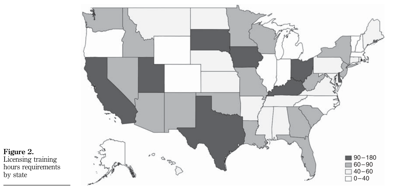 Figure 2. Open full-resolution image.
**Caption:** Licensing training hours requirements by state.
### 3.5 Estimated opportunity cost of training hours
As presented above, states vary in the required training hours. This variation is a large determinant of the variation in entry cost by state. Several techniques were explored regarding how to translate this variation into an economic measure of entry cost. The goal is to multiply the hours of training required by a measure of opportunity cost per hour.
One approach is to use a flat opportunity cost such as the minimum wage. This is the method employed in Zapletal (2017) while investigating cosmetologist licensing. (The results presented below are qualitatively robust to this approach). The method used here attempts to find a more precise estimate of the opportunity cost of new real estate agents. The hourly estimate found for each state is multiplied by the hours of training required in order to obtain a varying measure of training costs across states.
The opportunity cost for each state and each year are estimated from the 2011–2017 CPS (Flood et al., 2018). The CPS asks interview questions of respondents over a 16 month period on a rolling monthly basis. The interviews in the 4th and the 16th calendar months include additional information about income and employment. This sample includes 425,976 workers, of which 2,607 are real estate agents. This equates to 612 agents per 100,000 workers.
Of the 2,607 workers who report being a real estate agent in the follow-up interview, 503 report a different occupation one year earlier. The opportunity cost analysis uses these workers to determine new agents’ previous occupation category. A total of 24 percent of new agents reported being unemployed 12 months earlier. The most likely former occupations are manager, insurance sales and retail sales manager. The agents switched to real estate from a broad range of occupations but the most common broad category of switchers is sales occupations (Census codes 4700-4965), which is used as the control group in the regressions below.
Table IV shows the weekly earnings for sales workers. Many sales occupations, such as security sales agents and insurance agents, earn more than real estate agents do. This group also includes several low earning occupations, such as retail salespersons and cashiers. New agents who switched from a different occupation in the CPS are categorized as transitioning from one of four occupation categories: unemployment, low earning sales occupations, high earning sales occupations and other occupations. A total of 24 percent of agents switched from unemployment, 8 percent switched from high earning sales occupations, 7 percent from low earning sales occupations and 61 percent from a wide variety of other occupations.
### Table IV. Weekly earnings for sales occupations and fraction of new agents transitioning from each occupation
Figure 2. Open full-resolution image.
**Caption:** Licensing training hours requirements by state.
### 3.5 Estimated opportunity cost of training hours
As presented above, states vary in the required training hours. This variation is a large determinant of the variation in entry cost by state. Several techniques were explored regarding how to translate this variation into an economic measure of entry cost. The goal is to multiply the hours of training required by a measure of opportunity cost per hour.
One approach is to use a flat opportunity cost such as the minimum wage. This is the method employed in Zapletal (2017) while investigating cosmetologist licensing. (The results presented below are qualitatively robust to this approach). The method used here attempts to find a more precise estimate of the opportunity cost of new real estate agents. The hourly estimate found for each state is multiplied by the hours of training required in order to obtain a varying measure of training costs across states.
The opportunity cost for each state and each year are estimated from the 2011–2017 CPS (Flood et al., 2018). The CPS asks interview questions of respondents over a 16 month period on a rolling monthly basis. The interviews in the 4th and the 16th calendar months include additional information about income and employment. This sample includes 425,976 workers, of which 2,607 are real estate agents. This equates to 612 agents per 100,000 workers.
Of the 2,607 workers who report being a real estate agent in the follow-up interview, 503 report a different occupation one year earlier. The opportunity cost analysis uses these workers to determine new agents’ previous occupation category. A total of 24 percent of new agents reported being unemployed 12 months earlier. The most likely former occupations are manager, insurance sales and retail sales manager. The agents switched to real estate from a broad range of occupations but the most common broad category of switchers is sales occupations (Census codes 4700-4965), which is used as the control group in the regressions below.
Table IV shows the weekly earnings for sales workers. Many sales occupations, such as security sales agents and insurance agents, earn more than real estate agents do. This group also includes several low earning occupations, such as retail salespersons and cashiers. New agents who switched from a different occupation in the CPS are categorized as transitioning from one of four occupation categories: unemployment, low earning sales occupations, high earning sales occupations and other occupations. A total of 24 percent of agents switched from unemployment, 8 percent switched from high earning sales occupations, 7 percent from low earning sales occupations and 61 percent from a wide variety of other occupations.
### Table IV. Weekly earnings for sales occupations and fraction of new agents transitioning from each occupation
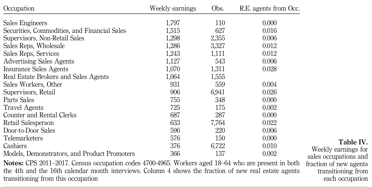 Table IV. Open full-resolution image.
Since workers in the CPS are interviewed for two years (Year 1 and Year 2), a comparison can be made between a new real estate agent’s earnings in his or her previous job in Year 1 and the earnings of their peers in Year 1. For example, if a worker reported being a new real estate agent in Year 2, one can compare their previous earnings from Year 1 (when they were a retail salesperson, for instance) to the average earnings of all retail salespeople in Year 1. On average, new real estate agents in Year 2, whose previous occupations were low-earning sales jobs in Year 1, earned higher wages in Year 1 than the average low-earning sales employee. However, if new real estate agents’ previous jobs in Year 1 were
high-earning sales jobs, they earned less on average than the median workers in the same occupation group in Year 1. New agents whose previous jobs in Year 1 were non-sales occupations earned slightly higher than average wages in their previous jobs before transitioning to becoming real estate agents.
Given this information, an opportunity cost per hour is calculated as a weighted average of the worker’s expected previous earnings. This value is calculated from the expected earnings premium over their peers: 1.48 for low earning sales occupations, 0.8 for high earning sales occupations, and 1.12 for other occupations. The factors are then multiplied by the median earnings for each occupation bin for each state and also multiplied by the transition probability. This implies that workers from lower income states will have lower estimated opportunity cost.
With the exception of DC ($25.28/hour), states range in opportunity cost from $14.79/hour (Mississippi) to $20.64/hour (Connecticut). The total opportunity cost is then obtained by multiplying this hourly opportunity cost by the total hours of training required in the state. Wyoming has the lowest total opportunity cost of training at $509 and Texas has the highest at $2,845. This is primarily driven by the difference in required training hours: 180 h in Texas and 30 h in Wyoming. The median total opportunity cost of training hours is $1,234.
It is important to note that this paper has not included potential reciprocity agreements among states. Many states offer a reduction or waiver for the required training hours for new agents transferring from another state. Reciprocity is particularly difficult to incorporate in this context, since some states have vague guidelines and all states with reciprocity only offer a partial reduction in costs. (The level of reciprocity may be dependent on the applicants originating state.) While this may reduce the marginal cost of out of state agents entering the new market, the investigation conducted for this paper suggests that reciprocity may play a small role in this industry. Less than 2 percent of real estate agent’s relocate to another state, which is
less than other professions, including other licensed professions. In addition, estimates (not shown) suggest that agents are no more likely than other occupations to relocate to another state when housing prices are increasing. This deterrent to moving may originate from the large social costs associated with becoming an agent in terms of developing a local client base and learning about the community. New agents are more likely to be local residents who become real estate agents, transitioning from other professions.
Additionally, the analysis has not incorporated a measurement of pass rates for new agents taking exams. While this is an interesting research agenda and has been discussed in the previous literature, pass rates for the majority of states are not publicly available to the authors’ knowledge. Estimates from data collected from nine states suggest first time pass rates may range from 50 to 70 percent and final pass rates may be around 85 percent. To the extent pass rates differ by state, aspiring agents may have differential expectations of the total licensing cost. This may play a limited role in the analysis here, given the potential lack of salience since most states do not disclose pass rates, and variation may be modest. Finally, geographic fixed effects could potentially control for time invariant differences in exam difficulty across states.
### 3.6 Housing and real estate agent data
Housing data are collected from the FHFA’s Quarterly All-Transactions Indexes. This provides a local index of single family home prices for each CBSA. These indexes are calculated from sales transaction data as well as appraisal data. The 100 largest CBSAs are used to avoid small samples associated with the number of real estate agents in other areas. Metro areas that lie in multiple states are also excluded from the analysis to avoid potential measurement issues with agents licensed and working in multiple states.
The housing prices are linked to workers in CBSAs using the ACS for 2012–2017. These years are selected to avoid the reclassification of occupations and CBSA boundaries occurring from 2011 to 2012. The sample is restricted to individuals 18–64 who have worked in the last 12 months and have a non-imputed occupation. The control group for the primary analysis is the Census broad occupation category of sales workers. These are Census occupation codes 4,700–4,965 (listed in Table III). The summary statistics are shown in Table V.
## 4. Results
The analysis below estimates the responsiveness of the real estate agent labor market to housing price increases and the associated impact of occupational licensing on labor market dynamics. As discussed in previous sections, an important barrier to entry in this profession is occupational licensing. Even though entry costs may be relatively small, studying this occupation allows for the analysis of entry barriers, given previous research showing agent entry is positively influenced by house price appreciation.
The goal of the empirical design is to estimate the effect of housing market changes, within a metro area, on the number of real estate agents, and to compare agent entry in metros with different licensing costs. The model assumes metro area housing prices are exogenous to agent entry. This is the assumption made in previous literature where empirical evidence suggests agents’ commissions are relatively fixed and aggregate housing appreciation implies an increase in potential earnings, inducing entry. This assumption is exploited in Barwick and Pathak (2015) using data from the Boston metro area and Hsieh and Moretti (2003) using national data.
The framework in this paper also aligns with the empirical real estate literature, which has primarily emphasized property and land characteristics in determining individual home values (Case and Quigley, 1991). Glaeser et al. (2005) additionally stress the importance of a non-increasing housing supply via building restrictions as a determinant of aggregate housing appreciation within metro areas. Their model assumes home values are driven by an increase in demand from consumer preferences paired with a lack of new development.
### Table V. Summary statistics: ACS linked to the FHFA metro housing index
Table IV. Open full-resolution image.
Since workers in the CPS are interviewed for two years (Year 1 and Year 2), a comparison can be made between a new real estate agent’s earnings in his or her previous job in Year 1 and the earnings of their peers in Year 1. For example, if a worker reported being a new real estate agent in Year 2, one can compare their previous earnings from Year 1 (when they were a retail salesperson, for instance) to the average earnings of all retail salespeople in Year 1. On average, new real estate agents in Year 2, whose previous occupations were low-earning sales jobs in Year 1, earned higher wages in Year 1 than the average low-earning sales employee. However, if new real estate agents’ previous jobs in Year 1 were
high-earning sales jobs, they earned less on average than the median workers in the same occupation group in Year 1. New agents whose previous jobs in Year 1 were non-sales occupations earned slightly higher than average wages in their previous jobs before transitioning to becoming real estate agents.
Given this information, an opportunity cost per hour is calculated as a weighted average of the worker’s expected previous earnings. This value is calculated from the expected earnings premium over their peers: 1.48 for low earning sales occupations, 0.8 for high earning sales occupations, and 1.12 for other occupations. The factors are then multiplied by the median earnings for each occupation bin for each state and also multiplied by the transition probability. This implies that workers from lower income states will have lower estimated opportunity cost.
With the exception of DC ($25.28/hour), states range in opportunity cost from $14.79/hour (Mississippi) to $20.64/hour (Connecticut). The total opportunity cost is then obtained by multiplying this hourly opportunity cost by the total hours of training required in the state. Wyoming has the lowest total opportunity cost of training at $509 and Texas has the highest at $2,845. This is primarily driven by the difference in required training hours: 180 h in Texas and 30 h in Wyoming. The median total opportunity cost of training hours is $1,234.
It is important to note that this paper has not included potential reciprocity agreements among states. Many states offer a reduction or waiver for the required training hours for new agents transferring from another state. Reciprocity is particularly difficult to incorporate in this context, since some states have vague guidelines and all states with reciprocity only offer a partial reduction in costs. (The level of reciprocity may be dependent on the applicants originating state.) While this may reduce the marginal cost of out of state agents entering the new market, the investigation conducted for this paper suggests that reciprocity may play a small role in this industry. Less than 2 percent of real estate agent’s relocate to another state, which is
less than other professions, including other licensed professions. In addition, estimates (not shown) suggest that agents are no more likely than other occupations to relocate to another state when housing prices are increasing. This deterrent to moving may originate from the large social costs associated with becoming an agent in terms of developing a local client base and learning about the community. New agents are more likely to be local residents who become real estate agents, transitioning from other professions.
Additionally, the analysis has not incorporated a measurement of pass rates for new agents taking exams. While this is an interesting research agenda and has been discussed in the previous literature, pass rates for the majority of states are not publicly available to the authors’ knowledge. Estimates from data collected from nine states suggest first time pass rates may range from 50 to 70 percent and final pass rates may be around 85 percent. To the extent pass rates differ by state, aspiring agents may have differential expectations of the total licensing cost. This may play a limited role in the analysis here, given the potential lack of salience since most states do not disclose pass rates, and variation may be modest. Finally, geographic fixed effects could potentially control for time invariant differences in exam difficulty across states.
### 3.6 Housing and real estate agent data
Housing data are collected from the FHFA’s Quarterly All-Transactions Indexes. This provides a local index of single family home prices for each CBSA. These indexes are calculated from sales transaction data as well as appraisal data. The 100 largest CBSAs are used to avoid small samples associated with the number of real estate agents in other areas. Metro areas that lie in multiple states are also excluded from the analysis to avoid potential measurement issues with agents licensed and working in multiple states.
The housing prices are linked to workers in CBSAs using the ACS for 2012–2017. These years are selected to avoid the reclassification of occupations and CBSA boundaries occurring from 2011 to 2012. The sample is restricted to individuals 18–64 who have worked in the last 12 months and have a non-imputed occupation. The control group for the primary analysis is the Census broad occupation category of sales workers. These are Census occupation codes 4,700–4,965 (listed in Table III). The summary statistics are shown in Table V.
## 4. Results
The analysis below estimates the responsiveness of the real estate agent labor market to housing price increases and the associated impact of occupational licensing on labor market dynamics. As discussed in previous sections, an important barrier to entry in this profession is occupational licensing. Even though entry costs may be relatively small, studying this occupation allows for the analysis of entry barriers, given previous research showing agent entry is positively influenced by house price appreciation.
The goal of the empirical design is to estimate the effect of housing market changes, within a metro area, on the number of real estate agents, and to compare agent entry in metros with different licensing costs. The model assumes metro area housing prices are exogenous to agent entry. This is the assumption made in previous literature where empirical evidence suggests agents’ commissions are relatively fixed and aggregate housing appreciation implies an increase in potential earnings, inducing entry. This assumption is exploited in Barwick and Pathak (2015) using data from the Boston metro area and Hsieh and Moretti (2003) using national data.
The framework in this paper also aligns with the empirical real estate literature, which has primarily emphasized property and land characteristics in determining individual home values (Case and Quigley, 1991). Glaeser et al. (2005) additionally stress the importance of a non-increasing housing supply via building restrictions as a determinant of aggregate housing appreciation within metro areas. Their model assumes home values are driven by an increase in demand from consumer preferences paired with a lack of new development.
### Table V. Summary statistics: ACS linked to the FHFA metro housing index
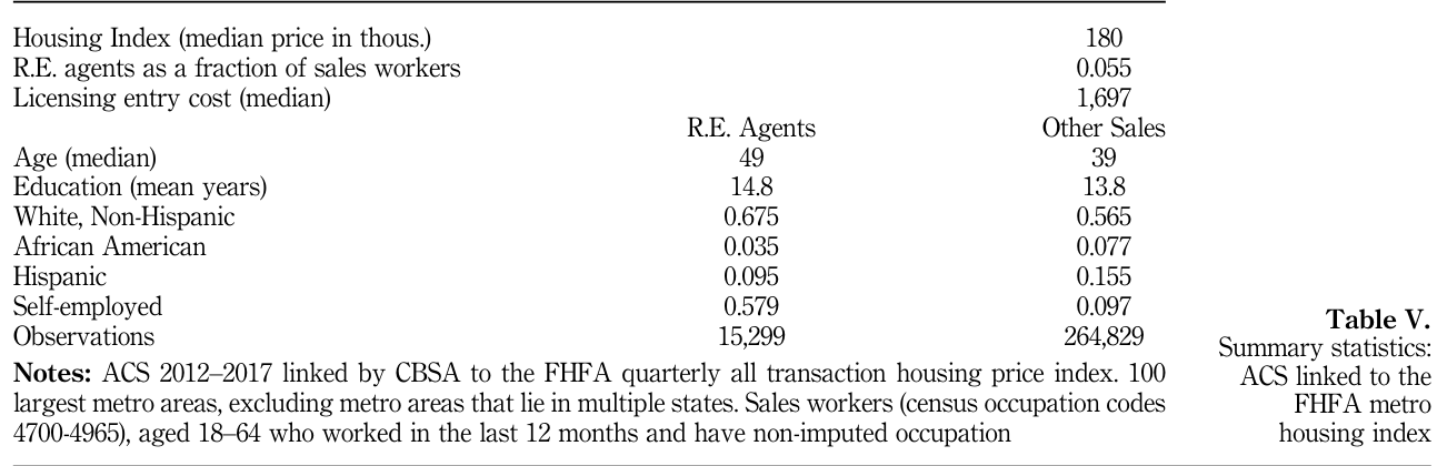 Table V. Open full-resolution image.
These building restrictions are potentially fully reflected in home values. Additionally, the estimation below includes CBSA fixed effects as well as specifications with and without population controls to test the sensitivity in this dimension. Population is controlled for by including the total number of respondents from all occupations, for a given metro area, for each survey year.
An important limitation in licensing studies is the cross-sectional nature of relatively unchanged licensing policies. Interacting licensing costs with housing appreciation enables the estimation of the licensing impact on labor market response using the exogenous year-over-year housing shocks. Unwanted correlation is still possible between existing licensing policies and future period labor elasticities. This analysis does not have the benefit of panel data for licensing changes but using constant licensing costs mitigates some concerns with respect to endogenous policy changes. In Equation (2), cross-sectional licensing policies are allowed to be correlated with the initial stock of agents, but the underlying assumption is that two cities with the same housing appreciation would experience a similar agent labor market response if they had identical
licensing costs, after controlling for observables. Year and CBSA fixed effects are included but unobserved correlation could still bias the results:
**Equation (2):**
**Equation (2)**
Table VI shows the results from the estimation of Equation (2). if worker , in CBSA , in year , is a real estate agent and 0 otherwise. is the median housing price of CBSA in period .5 is the licensing entry cost for CBSA . Individual characteristics include binned age, binned education, sex, race, and ethnicity. Fixed effects for CBSA () and year () are included. Specification 2 controls for population (). Errors are clustered at the CBSA level. The control group is 18–64-year-old sales workers in the respective metro areas.6
### Table VI. The effect of housing price appreciation and licensing costs on real estate agent entry
Table V. Open full-resolution image.
These building restrictions are potentially fully reflected in home values. Additionally, the estimation below includes CBSA fixed effects as well as specifications with and without population controls to test the sensitivity in this dimension. Population is controlled for by including the total number of respondents from all occupations, for a given metro area, for each survey year.
An important limitation in licensing studies is the cross-sectional nature of relatively unchanged licensing policies. Interacting licensing costs with housing appreciation enables the estimation of the licensing impact on labor market response using the exogenous year-over-year housing shocks. Unwanted correlation is still possible between existing licensing policies and future period labor elasticities. This analysis does not have the benefit of panel data for licensing changes but using constant licensing costs mitigates some concerns with respect to endogenous policy changes. In Equation (2), cross-sectional licensing policies are allowed to be correlated with the initial stock of agents, but the underlying assumption is that two cities with the same housing appreciation would experience a similar agent labor market response if they had identical
licensing costs, after controlling for observables. Year and CBSA fixed effects are included but unobserved correlation could still bias the results:
**Equation (2):**
**Equation (2)**
Table VI shows the results from the estimation of Equation (2). if worker , in CBSA , in year , is a real estate agent and 0 otherwise. is the median housing price of CBSA in period .5 is the licensing entry cost for CBSA . Individual characteristics include binned age, binned education, sex, race, and ethnicity. Fixed effects for CBSA () and year () are included. Specification 2 controls for population (). Errors are clustered at the CBSA level. The control group is 18–64-year-old sales workers in the respective metro areas.6
### Table VI. The effect of housing price appreciation and licensing costs on real estate agent entry
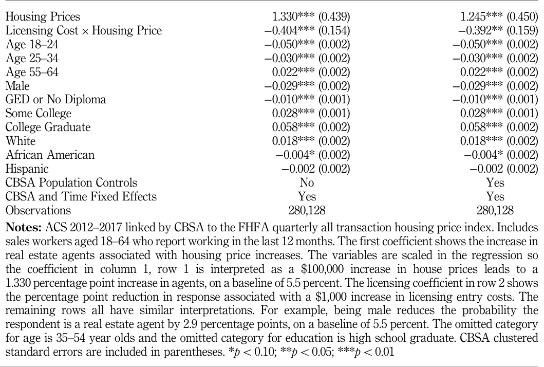 Table VI. Open full-resolution image.
The results are similar in specifications controlling for population changes and specifications using all workers. Robustness checks have also been conducted using metro area GDP and unemployment. The inclusion of these local economic variables are not significant in the regression and have small magnitudes, suggesting little unobserved residual variation in the local economy after controlling for metro and time effects.
Table VI shows that after controlling for licensing costs, a 10 percent increase in housing prices leads to a 4.1–4.4 percent increase in agents. The coefficient on the interaction of licensing and housing prices shows the effect of licensing on the labor response. The evidence suggests that licensing results in a meaningful reduction of agent entry. An additional $1,000 of licensing entry costs are associated with roughly a 30 percent reduction in labor response. (Alternatively, a one standard deviation increase in licensing cost is associated with 24 percent less agent entry). Results also show the probability of being a real estate agent increases with age, increases for females, increases with education and increases for respondents identifying as white, non-Hispanic.
Table VII shows the results with additional interactions for women and for workers less than 50 years old. The median age for real estate agents in the sample is 49, and younger workers may be more responsive to entry incentives and barriers. A $1,000 increase in licensing costs results in an 18 percent reduction in entry for workers over 50 years old and a 31 percent reduction in entry for younger workers. The estimate for the effect of licensing barriers on women is noisy but shows this subpopulation is more responsive to entry barriers in the real estate industry. The point estimates show women are more likely to become agents when home prices increase, but a $1,000 increase in licensing costs reduces the entry response
of women by roughly 50 percent. Women also show more responsiveness to entry barriers when splitting the sample and running the previous regressions on men and women separately.
Other specifications of the model find qualitatively similar results. Tables AI and AII show the results are robust to excluding the five states that are categorized in the national databases as being without explicit sales agent licensing. Tables AI and AII also include estimates showing the results are robust to using all occupations as the control group. In addition, the result is robust to estimating the model using the federal minimum wage as an opportunity cost for training hours. Following an estimation technique previously used in the real estate literature, but with the addition of licensing barriers, long-term labor responses have also been estimated. The difference between the percent of agents in the metro area in 2012 and 2017 is regressed on the difference in CBSA housing prices over these six years. A 10 percent increase in housing prices over the longer time horizon results in a 7 percent increase in agents, but $1,000 of additional licensing costs again reduce entry by 33 percent. This estimate aligns with previous work. The Boston data analyzed by Barwick and Pathak (2015) show an 8 percent increase in agents for a 10 percent increase in home values from 1998 to 2004. Hsieh and Moretti (2003) find that a 10 percent increase in home prices from 1980 to 1990 was associated with 7 percent more agents using the national Decennial Census data.
### Table VII. The effect of housing price appreciation and licensing costs on real estate agent entry
Table VI. Open full-resolution image.
The results are similar in specifications controlling for population changes and specifications using all workers. Robustness checks have also been conducted using metro area GDP and unemployment. The inclusion of these local economic variables are not significant in the regression and have small magnitudes, suggesting little unobserved residual variation in the local economy after controlling for metro and time effects.
Table VI shows that after controlling for licensing costs, a 10 percent increase in housing prices leads to a 4.1–4.4 percent increase in agents. The coefficient on the interaction of licensing and housing prices shows the effect of licensing on the labor response. The evidence suggests that licensing results in a meaningful reduction of agent entry. An additional $1,000 of licensing entry costs are associated with roughly a 30 percent reduction in labor response. (Alternatively, a one standard deviation increase in licensing cost is associated with 24 percent less agent entry). Results also show the probability of being a real estate agent increases with age, increases for females, increases with education and increases for respondents identifying as white, non-Hispanic.
Table VII shows the results with additional interactions for women and for workers less than 50 years old. The median age for real estate agents in the sample is 49, and younger workers may be more responsive to entry incentives and barriers. A $1,000 increase in licensing costs results in an 18 percent reduction in entry for workers over 50 years old and a 31 percent reduction in entry for younger workers. The estimate for the effect of licensing barriers on women is noisy but shows this subpopulation is more responsive to entry barriers in the real estate industry. The point estimates show women are more likely to become agents when home prices increase, but a $1,000 increase in licensing costs reduces the entry response
of women by roughly 50 percent. Women also show more responsiveness to entry barriers when splitting the sample and running the previous regressions on men and women separately.
Other specifications of the model find qualitatively similar results. Tables AI and AII show the results are robust to excluding the five states that are categorized in the national databases as being without explicit sales agent licensing. Tables AI and AII also include estimates showing the results are robust to using all occupations as the control group. In addition, the result is robust to estimating the model using the federal minimum wage as an opportunity cost for training hours. Following an estimation technique previously used in the real estate literature, but with the addition of licensing barriers, long-term labor responses have also been estimated. The difference between the percent of agents in the metro area in 2012 and 2017 is regressed on the difference in CBSA housing prices over these six years. A 10 percent increase in housing prices over the longer time horizon results in a 7 percent increase in agents, but $1,000 of additional licensing costs again reduce entry by 33 percent. This estimate aligns with previous work. The Boston data analyzed by Barwick and Pathak (2015) show an 8 percent increase in agents for a 10 percent increase in home values from 1998 to 2004. Hsieh and Moretti (2003) find that a 10 percent increase in home prices from 1980 to 1990 was associated with 7 percent more agents using the national Decennial Census data.
### Table VII. The effect of housing price appreciation and licensing costs on real estate agent entry
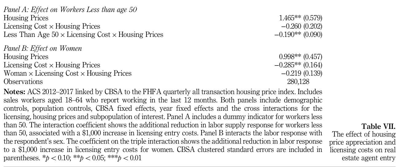 Table VII. Open full-resolution image.
## 5. Conclusion
This paper exploits the geographic variation in housing prices and licensing entry barriers to determine the impact of entry costs on labor market dynamics. In a labor market with arguably low entry barriers, the initial evidence suggests licensing costs still have significant employment effects. These results also suggest potential impacts of occupational licensing on entrepreneurship, given the high level of self-employment in this occupation. The geographic documentation of licensing costs additionally provides insights into the heterogenous licensing policies in this industry and the impacts of these regulations across states.
At a first pass, a 30 percent reduction in labor response seems disproportionally large for a $1,000 increase in entry costs. There are several reasons why entry barriers may play an outsized role here, beyond the potential limitations in estimation discussed in Sections 3 and 4. First, these entry costs do not capture potentially ongoing regulatory burdens and continuing education that may act as a compounding deterrent. These ongoing regulatory costs are likely correlated with entry costs. In addition, licensing costs are disproportionally burdensome to new agents and agents at the margin of entry who have lower average earnings than incumbents do. This also applies to potential entrants who are looking for supplementary income or agents looking to enter the industry for a limited
time. Licensing is a fixed yearly cost that will discourage workers anticipating a limited number of sales.
The discussion so far has also assumed perfect information. An important issue for real estate sales is the learning new agents uncover about their own ability. Barwick and Pathak (2015) stress the heterogeneity of licensed agents, but this heterogeneity may play an equal or more important role for workers deciding whether to become licensed. The uncertainty coupled with the initial required investment may dissuade risk-averse entrants and may persuade entrepreneurs to substitute into other industries.
In terms of welfare, the previous literature has highlighted potential losses in efficiency from free entry into the real estate profession. This arises either from agents of lower ability entering in markets with lower barriers or from a dispersion of clients, making each agent less productive in terms of total sales. The first point arises from a Leland’s (1979) framework where licensing barriers screen out the lowest quality entrants. This argument assumes licensing barriers are more likely to screen out the worst potential entrants and assumes agents have full information about their own ability. An alternative argument was raised in Angrist and Guryan (2008) when investigating if teacher licensing screens out the worst candidates. If high quality candidates have more career choices,
increasing entry barriers shift the best quality applicants into less costly professions at the margin. Finally, the welfare analyses in previous studies assume a fixed cost of doing business, where average total cost is reduced with more sales. Lower licensing requirements may allow for more part-time, “gig economy” agents or more innovative entrepreneurship, potentially reducing the fixed cost of doing business, in a similar manner as the taxi industry.
As an additional note, real estate licensing, like many licensing regimes, varies greatly across states. This implies that some states likely have room for welfare gains for either agents or homebuyers. Intrastate welfare may also suffer from these homogeneous licensing policies applied to heterogenous regions in the state. Both the labor and housing market vary greatly between urban and rural settings. The focus in this paper has been on the impact of licensing policies on urban real estate agents in the largest metro areas, where better data are available. Future investigations may conclude licensing has more or less impact in dampening the labor response in non-urban markets.
In terms of actionable policy implications, this paper has highlighted several margins for potential reductions in entry barriers. As discussed above, reciprocity agreements may offer limited benefit in the real estate industry, compared to industries with less required geographic investment. Comparing the proportion of total costs derived from fees, course tuition and hours of training required, the largest component – and the component driving the largest variation across states – is the required hours of training. Approximately 9 percent of the total cost of licensing is derived from fees, 21 percent is derived from course tuition, and 70 percent is derived from the hours requirement, which varies from 30 to 180 h. This is the difference between a two- or three-weekend seminar and a six-month formal training.
As an illustrative example, if all states reduced the required hours to 40, the estimated total cost of licensing would drop from an approximate range of $1,000–3,500 to a range of $700–1,850. It would also significantly reduce the total calendar time it takes to get a license in many states and would likely reduce the tuition charged by real estate schools.
While the focus of this study is the effect of entry barriers on labor supply, the analysis has not incorporated the potential effects of reducing required hours of training on service quality. The investigation of this issue has been introduced in the previous real estate licensing literature, but the impacts of licensing restrictions on service quality is still an ongoing area of research, suggesting potential for future work. With respect to entry barriers, however, the results presented here suggest reducing entry frictions would increase the number of workers in the profession. This has implications for unemployment, as 24 percent of new agents are transitioning from unemployment, as well as for entrepreneurship and dynamism, as 58 percent of agents are self-employed. The results
also suggest a reduction in barriers may have larger effects on women and younger workers, demographics some states may hope to target for employment policies and entrepreneurship. These state policies, as well as similar licensing policies in other professions, may provide states a path forward to increase state dynamism, promote entrepreneurship, and decrease unemployment.
## References
- Angrist, J.D. and Guryan, J. (2008), “Does teacher testing raise teacher quality? Evidence from state certification requirements”, Economics of Education Review, Vol. 27 No. 5, pp. 483-503.
- Barwick, P.J. and Pathak, P.A. (2015), “The costs of free entry: an empirical study of real estate agents in greater Boston”, The RAND Journal of Economics, Vol. 46 No. 1, pp. 103-145.
- Beck, J., Scott, F. and Yelowitz, A. (2012), “Concentration and market structure in local real estate markets”, Real Estate Economics, Vol. 40 No. 3, pp. 422-460.
- Blair, P.Q. and Chung, B.W. (2018), “How much of a barrier to entry is occupational licensing?”, Working Paper No. 25262, NBER, Cambridge, MA, November.
- Carroll, S.L. and Gaston, R.J. (1983), “Occupational licensing and the quality of service: an overview”, Law and Human Behavior, Vol. 7 Nos 2/3, pp. 139-146.
- Case, B. and Quigley, J.M. (1991), “The dynamics of real estate prices”, The Review of Economics and Statistics, Vol. 73 No. 1, pp. 50-58.
- Cathles, A., Harrington, D.E. and Krynski, K. (2010), “The gender gap in funeral directors: burying women with ready-to-embalm laws?”, British Journal of Industrial Relations, Vol. 48 No. 4, pp. 688-705.
- Cebula, R.J., Connaughton, J. and Swartz, C. (2018), “An empirical analysis of the impact of the three labor market freedom indices and occupational licensing on interstate living-cost differentials”, The Journal of Private Enterprise, Vol. 33 No. 2, pp. 49-62.
- CSOR (2019), “Occupational Licensing Database”, Knee Center for the Study of Occupational Regulation, Loretto, PA, available at: https://csorsfu.com
- Flood, S., King, M., Rodgers, R., Ruggles, S. and Warren, J.R. (2018), “Integrated public use microdata series, Current Population Survey: version 6.0 [dataset]”, IPUMS, Minneapolis, MN, available at: https://doi.org/10.18128/D030.V6.0
- Glaeser, E.L., Gyourko, J. and Saks, R.E. (2005), “Why have housing prices gone up?”, The American Economic Review, Vol. 95 No. 2, pp. 329-333.
- Goldschlag, N. and Tabarrok, A. (2018), “Is regulation to blame for the decline in American entrepreneurship?”, Economic Policy, Vol. 33 No. 93, pp. 5-44.
- Guntermann, K.L. and Smith, R.L. (1988), “Licensing requirements, enforcement effort, and complaints against real estate agents”, The Journal of Real Estate Research, Vol. 3 No. 2, pp. 11-20.
- Hsieh, C. and Moretti, E. (2003), “Can free entry be inefficient? Fixed commissions and social waste in the real estate industry”, Journal of Political Economy, Vol. 111 No. 5, pp. 1076-1122.
- Johnson, L.L. and Loucks, C. (1986), “The effect of state licensing regulations on the real estate brokerage industry”, American Real Estate and Urban Economics Association Journal, Vol. 14 No. 4, pp. 567-582.
- Kleiner, M.M. (2006), Licensing Occupations: Ensuring Quality or Restricting Competition?, W.E. Upjohn Institute for Employment Research, Kalamazoo, MI.
- Kleiner, M.M. and Kudrle, R. (2000), “Does regulation affect economic outcomes? The case of dentistry”, The Journal of Law and Economics, Vol. 43 No. 2, pp. 547-582.
- Kleiner, M.M. and Soltas, E. (2019), “A welfare analysis of occupational licensing in U.S. states”, paper presented at the Allied Social Science Association Annual Meeting, Atlanta, GA, January.
- Leland, H.E. (1979), “Quacks, lemons, and licensing: a theory of minimum quality standards”, Journal of Political Economy, Vol. 87 No. 6, pp. 1328-1346.
- Mellor, W. and Carpenter, D.M. (2016), Bottleneckers: Gaming the Government for Power and Private Profit, Encounter Books, New York, NY.
- NAR (2019), “Quick Real Estate Statistics”, National Association of Realtors, Washington, DC, available at: www.nar.realtor (accessed April 2019).
- NCSL (2019), “The National Occupational Licensing Database”, National Council of State Legislatures, Washington, DC, available at: www.ncsl.org
- Neumark, D. and Wascher, W. (2008), Minimum Wages, MIT Press, Cambridge, MA.
- Powell, B. and Vorotnikov, E.S. (2012), “Real estate continuing education: rent seeking or improvement in service quality?”, Eastern Economic Journal, Vol. 38 No. 1, pp. 57-73.
- Prantl, S. and Spitz-Oener, A. (2009), “How does entry regulation influence entry into self-employment mobility?”, Economics of Transition, Vol. 17 No. 4, pp. 769-802.
- Shilling, J.D. and Sirmans, C.F. (1988), “The effects of occupational licensing on complaints against real estate agents”, The Journal of Real Estate Research, Vol. 3 No. 2, pp. 1-9.
- Slivinksi, S. (2015), “Bootstraps tangles in red tape: how state occupational licensing hinders low-income entrepreneurship”, Goldwater Institute Policy Report No. 272, Phoenix, AZ, available at: https://goldwaterinstitute.org (accessed April 2019).
- Stephenson, E.F. and Meehan, B. (2018), “Accounting for the impact of the 120/150 CPA licensing rule”, paper presented at the Southern Economic Association Annual Meeting, Washington DC, November.
- Thornton, R.J. and Timmons, E.J. (2013), “Licensing one of the world’s oldest professions: massage”, Journal of Law and Economics, Vol. 56 No. 2, pp. 371-388.
- Vorotnikov, E.S. (2011), “License to profit: an analysis of entry regulations in the legal and real estate professions”, University of St. Thomas Journal of Law and Public Policy, Vol. 5 No. 2, pp. 52-66.
- Wiens, J. and Jackson, C. (2015), “Occupational licensing: a barrier to entrepreneurship”, available at: https://kauffman.org (accessed July 1, 2018).
- Zapletal, M. (2017), “The effects of occupational licensing evidence from detailed business-level data”, Working Paper No. CES-WP-17-20, US Census Bureau Center for Economic Studies, Washington DC, February.
## Appendix
### Table AI. Housing price appreciation and real estate agent entry: omitting five states without licensing
Table VII. Open full-resolution image.
## 5. Conclusion
This paper exploits the geographic variation in housing prices and licensing entry barriers to determine the impact of entry costs on labor market dynamics. In a labor market with arguably low entry barriers, the initial evidence suggests licensing costs still have significant employment effects. These results also suggest potential impacts of occupational licensing on entrepreneurship, given the high level of self-employment in this occupation. The geographic documentation of licensing costs additionally provides insights into the heterogenous licensing policies in this industry and the impacts of these regulations across states.
At a first pass, a 30 percent reduction in labor response seems disproportionally large for a $1,000 increase in entry costs. There are several reasons why entry barriers may play an outsized role here, beyond the potential limitations in estimation discussed in Sections 3 and 4. First, these entry costs do not capture potentially ongoing regulatory burdens and continuing education that may act as a compounding deterrent. These ongoing regulatory costs are likely correlated with entry costs. In addition, licensing costs are disproportionally burdensome to new agents and agents at the margin of entry who have lower average earnings than incumbents do. This also applies to potential entrants who are looking for supplementary income or agents looking to enter the industry for a limited
time. Licensing is a fixed yearly cost that will discourage workers anticipating a limited number of sales.
The discussion so far has also assumed perfect information. An important issue for real estate sales is the learning new agents uncover about their own ability. Barwick and Pathak (2015) stress the heterogeneity of licensed agents, but this heterogeneity may play an equal or more important role for workers deciding whether to become licensed. The uncertainty coupled with the initial required investment may dissuade risk-averse entrants and may persuade entrepreneurs to substitute into other industries.
In terms of welfare, the previous literature has highlighted potential losses in efficiency from free entry into the real estate profession. This arises either from agents of lower ability entering in markets with lower barriers or from a dispersion of clients, making each agent less productive in terms of total sales. The first point arises from a Leland’s (1979) framework where licensing barriers screen out the lowest quality entrants. This argument assumes licensing barriers are more likely to screen out the worst potential entrants and assumes agents have full information about their own ability. An alternative argument was raised in Angrist and Guryan (2008) when investigating if teacher licensing screens out the worst candidates. If high quality candidates have more career choices,
increasing entry barriers shift the best quality applicants into less costly professions at the margin. Finally, the welfare analyses in previous studies assume a fixed cost of doing business, where average total cost is reduced with more sales. Lower licensing requirements may allow for more part-time, “gig economy” agents or more innovative entrepreneurship, potentially reducing the fixed cost of doing business, in a similar manner as the taxi industry.
As an additional note, real estate licensing, like many licensing regimes, varies greatly across states. This implies that some states likely have room for welfare gains for either agents or homebuyers. Intrastate welfare may also suffer from these homogeneous licensing policies applied to heterogenous regions in the state. Both the labor and housing market vary greatly between urban and rural settings. The focus in this paper has been on the impact of licensing policies on urban real estate agents in the largest metro areas, where better data are available. Future investigations may conclude licensing has more or less impact in dampening the labor response in non-urban markets.
In terms of actionable policy implications, this paper has highlighted several margins for potential reductions in entry barriers. As discussed above, reciprocity agreements may offer limited benefit in the real estate industry, compared to industries with less required geographic investment. Comparing the proportion of total costs derived from fees, course tuition and hours of training required, the largest component – and the component driving the largest variation across states – is the required hours of training. Approximately 9 percent of the total cost of licensing is derived from fees, 21 percent is derived from course tuition, and 70 percent is derived from the hours requirement, which varies from 30 to 180 h. This is the difference between a two- or three-weekend seminar and a six-month formal training.
As an illustrative example, if all states reduced the required hours to 40, the estimated total cost of licensing would drop from an approximate range of $1,000–3,500 to a range of $700–1,850. It would also significantly reduce the total calendar time it takes to get a license in many states and would likely reduce the tuition charged by real estate schools.
While the focus of this study is the effect of entry barriers on labor supply, the analysis has not incorporated the potential effects of reducing required hours of training on service quality. The investigation of this issue has been introduced in the previous real estate licensing literature, but the impacts of licensing restrictions on service quality is still an ongoing area of research, suggesting potential for future work. With respect to entry barriers, however, the results presented here suggest reducing entry frictions would increase the number of workers in the profession. This has implications for unemployment, as 24 percent of new agents are transitioning from unemployment, as well as for entrepreneurship and dynamism, as 58 percent of agents are self-employed. The results
also suggest a reduction in barriers may have larger effects on women and younger workers, demographics some states may hope to target for employment policies and entrepreneurship. These state policies, as well as similar licensing policies in other professions, may provide states a path forward to increase state dynamism, promote entrepreneurship, and decrease unemployment.
## References
- Angrist, J.D. and Guryan, J. (2008), “Does teacher testing raise teacher quality? Evidence from state certification requirements”, Economics of Education Review, Vol. 27 No. 5, pp. 483-503.
- Barwick, P.J. and Pathak, P.A. (2015), “The costs of free entry: an empirical study of real estate agents in greater Boston”, The RAND Journal of Economics, Vol. 46 No. 1, pp. 103-145.
- Beck, J., Scott, F. and Yelowitz, A. (2012), “Concentration and market structure in local real estate markets”, Real Estate Economics, Vol. 40 No. 3, pp. 422-460.
- Blair, P.Q. and Chung, B.W. (2018), “How much of a barrier to entry is occupational licensing?”, Working Paper No. 25262, NBER, Cambridge, MA, November.
- Carroll, S.L. and Gaston, R.J. (1983), “Occupational licensing and the quality of service: an overview”, Law and Human Behavior, Vol. 7 Nos 2/3, pp. 139-146.
- Case, B. and Quigley, J.M. (1991), “The dynamics of real estate prices”, The Review of Economics and Statistics, Vol. 73 No. 1, pp. 50-58.
- Cathles, A., Harrington, D.E. and Krynski, K. (2010), “The gender gap in funeral directors: burying women with ready-to-embalm laws?”, British Journal of Industrial Relations, Vol. 48 No. 4, pp. 688-705.
- Cebula, R.J., Connaughton, J. and Swartz, C. (2018), “An empirical analysis of the impact of the three labor market freedom indices and occupational licensing on interstate living-cost differentials”, The Journal of Private Enterprise, Vol. 33 No. 2, pp. 49-62.
- CSOR (2019), “Occupational Licensing Database”, Knee Center for the Study of Occupational Regulation, Loretto, PA, available at: https://csorsfu.com
- Flood, S., King, M., Rodgers, R., Ruggles, S. and Warren, J.R. (2018), “Integrated public use microdata series, Current Population Survey: version 6.0 [dataset]”, IPUMS, Minneapolis, MN, available at: https://doi.org/10.18128/D030.V6.0
- Glaeser, E.L., Gyourko, J. and Saks, R.E. (2005), “Why have housing prices gone up?”, The American Economic Review, Vol. 95 No. 2, pp. 329-333.
- Goldschlag, N. and Tabarrok, A. (2018), “Is regulation to blame for the decline in American entrepreneurship?”, Economic Policy, Vol. 33 No. 93, pp. 5-44.
- Guntermann, K.L. and Smith, R.L. (1988), “Licensing requirements, enforcement effort, and complaints against real estate agents”, The Journal of Real Estate Research, Vol. 3 No. 2, pp. 11-20.
- Hsieh, C. and Moretti, E. (2003), “Can free entry be inefficient? Fixed commissions and social waste in the real estate industry”, Journal of Political Economy, Vol. 111 No. 5, pp. 1076-1122.
- Johnson, L.L. and Loucks, C. (1986), “The effect of state licensing regulations on the real estate brokerage industry”, American Real Estate and Urban Economics Association Journal, Vol. 14 No. 4, pp. 567-582.
- Kleiner, M.M. (2006), Licensing Occupations: Ensuring Quality or Restricting Competition?, W.E. Upjohn Institute for Employment Research, Kalamazoo, MI.
- Kleiner, M.M. and Kudrle, R. (2000), “Does regulation affect economic outcomes? The case of dentistry”, The Journal of Law and Economics, Vol. 43 No. 2, pp. 547-582.
- Kleiner, M.M. and Soltas, E. (2019), “A welfare analysis of occupational licensing in U.S. states”, paper presented at the Allied Social Science Association Annual Meeting, Atlanta, GA, January.
- Leland, H.E. (1979), “Quacks, lemons, and licensing: a theory of minimum quality standards”, Journal of Political Economy, Vol. 87 No. 6, pp. 1328-1346.
- Mellor, W. and Carpenter, D.M. (2016), Bottleneckers: Gaming the Government for Power and Private Profit, Encounter Books, New York, NY.
- NAR (2019), “Quick Real Estate Statistics”, National Association of Realtors, Washington, DC, available at: www.nar.realtor (accessed April 2019).
- NCSL (2019), “The National Occupational Licensing Database”, National Council of State Legislatures, Washington, DC, available at: www.ncsl.org
- Neumark, D. and Wascher, W. (2008), Minimum Wages, MIT Press, Cambridge, MA.
- Powell, B. and Vorotnikov, E.S. (2012), “Real estate continuing education: rent seeking or improvement in service quality?”, Eastern Economic Journal, Vol. 38 No. 1, pp. 57-73.
- Prantl, S. and Spitz-Oener, A. (2009), “How does entry regulation influence entry into self-employment mobility?”, Economics of Transition, Vol. 17 No. 4, pp. 769-802.
- Shilling, J.D. and Sirmans, C.F. (1988), “The effects of occupational licensing on complaints against real estate agents”, The Journal of Real Estate Research, Vol. 3 No. 2, pp. 1-9.
- Slivinksi, S. (2015), “Bootstraps tangles in red tape: how state occupational licensing hinders low-income entrepreneurship”, Goldwater Institute Policy Report No. 272, Phoenix, AZ, available at: https://goldwaterinstitute.org (accessed April 2019).
- Stephenson, E.F. and Meehan, B. (2018), “Accounting for the impact of the 120/150 CPA licensing rule”, paper presented at the Southern Economic Association Annual Meeting, Washington DC, November.
- Thornton, R.J. and Timmons, E.J. (2013), “Licensing one of the world’s oldest professions: massage”, Journal of Law and Economics, Vol. 56 No. 2, pp. 371-388.
- Vorotnikov, E.S. (2011), “License to profit: an analysis of entry regulations in the legal and real estate professions”, University of St. Thomas Journal of Law and Public Policy, Vol. 5 No. 2, pp. 52-66.
- Wiens, J. and Jackson, C. (2015), “Occupational licensing: a barrier to entrepreneurship”, available at: https://kauffman.org (accessed July 1, 2018).
- Zapletal, M. (2017), “The effects of occupational licensing evidence from detailed business-level data”, Working Paper No. CES-WP-17-20, US Census Bureau Center for Economic Studies, Washington DC, February.
## Appendix
### Table AI. Housing price appreciation and real estate agent entry: omitting five states without licensing
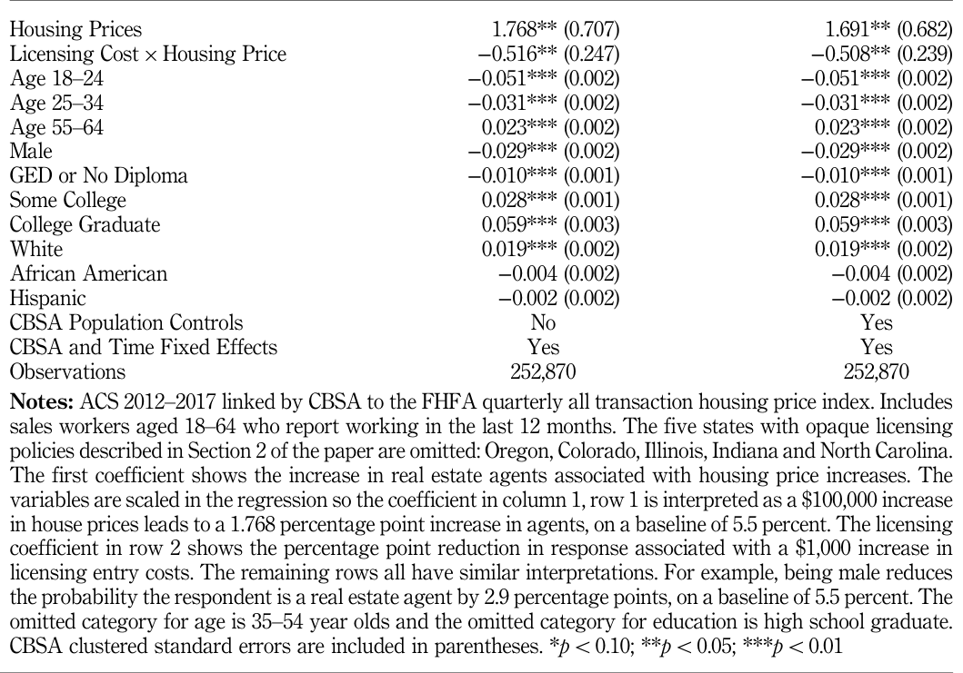 Table AI. Open full-resolution image.
### Table AII. Housing price appreciation and real estate agent entry: all occupations as control group
Table AI. Open full-resolution image.
### Table AII. Housing price appreciation and real estate agent entry: all occupations as control group
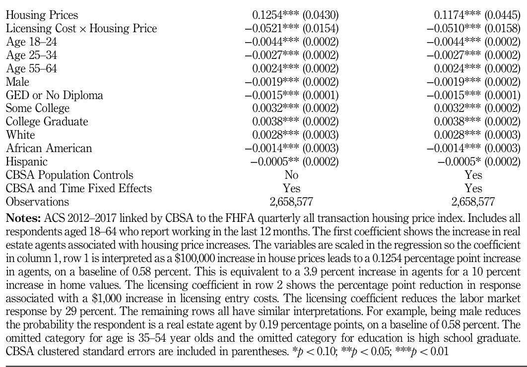 Table AII. Open full-resolution image.
## Corresponding author
Samuel J. Ingram can be contacted at: samuel.ingram@uky.edu
For instructions on how to order reprints of this article, please visit our website: www.emeraldgrouppublishing.com/licensing/reprints.htm
Or contact us for further details: permissions@emeraldinsight.com
---
## Notes
Table AII. Open full-resolution image.
## Corresponding author
Samuel J. Ingram can be contacted at: samuel.ingram@uky.edu
For instructions on how to order reprints of this article, please visit our website: www.emeraldgrouppublishing.com/licensing/reprints.htm
Or contact us for further details: permissions@emeraldinsight.com
---
## Notes
1. www.zillow.com/research/total-value-homes-31-8-trillion-17763/
2. www.nar.realtor/sites/default/files/documents/ehs-02-2019-single-family-only-2019-03-22.pdf
3. www.nar.realtor/research-and-statistics/quick-real-estate-statistics
4. DC will be informally referred to as a state, e.g. “51 states were analyzed.”
5. Housing markets have been shown to be local and Beck et al. (2012) note that metro areas are a good approximation to the scope of the market.
6. All occupations in the “Sales and Related Occupations” which are listed in order of earnings in Table III.